Click’s measurements are nice because they do a better job of separating a runner’s performance from the batters preceding and following him. Click described three different situations where a good base runner can get an extra base:

We can search for these situations in the play-by-play data and count the number of times each player reached the expected base and the extra base. The next step is to compare each player’s total to the league average.

First, we will use play-by-play data, as described in “Load Baseball Data into MySQL” [Hack #20] . Now, we want to calculate each base runner’s statistics in each situation. I’ll use a SQL trick to calculate these in one type of statement: a CASE statement. The idea is to perform a logical test on each line—for example, to check whether the play was a single with one runner on second. Then we set a column to 1 or 0, depending on whether the player reached the expected base or extra bases, and sum the totals by player. Here’s the code I used to count these situations, and to count the number of times each player got the expected number of bases and extra bases:

	create table pbp.baserunning2k as
	select year,
	 if(case1 OR case2, first_runner, second_runner) as pid,
	 sum(case1) as case1,
	 sum(if(runner_on_1st_dest>2 AND case1,1,0)) as case1_extra,
	 sum(case2) as case2,
	 sum(if(runner_on_1st_dest>3 AND case2,1,0)) as case2_extra,
	 sum(case3) as case3,
	 sum(if(runner_on_2nd_dest>3 AND case3,1,0)) as case3_extra,
	 group_concat(distinct teamID separator ',') as teamIDs
	from (select first_runner, second_runner, runner_on_1st_dest, runner_on_2nd_dest,
	 if(hit_value=1 AND first_runner != "" AND second_runner = "" AND third_runner = "",1,0) 
CASE1,
	 if(hit_value=2 AND first_runner != "" AND second_runner = "" AND third_runner = "",1,0) 
CASE2,
	 if(hit_value=2 AND second_runner != "" AND third_runner = "",1,0) CASE3,
	 if(batting_team=1, substr(game_id,1,3), visiting_team) teamID,
	 substr(game_id,4,4) as year
	 from  pbp2k) p
	where case1=1 or case2=1 or case3=1
	group by if(case1 OR case2, first_runner, second_runner), year;
	create index baserunning2k_idx on baserunning2k(year, pid);
	create index rosters_idx on rosters(year, retroID);

I wanted a percentage measurement, and not just an absolute number of extra runs, for each base runner. So I devised a measurement called extra base running percent (XBRpct) that measured the percentage of equivalent batter runs scored out of all opportunities. Here is the R code that I used to calculate XBRpct. (You’ll have to load the RODBC library and configure an ODBC connection called pbp to use this code.)

	# modify dbname, username, and password fields to match your database
	pbp.com <- dbConnect(drv, username="jadler",
	  dbname="retrosheet",host="localhost",
	  password="p@ssw0rd")
	baserunning.query <- dbSendQuery(pbp.con, statement = paste (
	  "SELECT l.*, r.lastName, r.firstName, r.team ",
	  "from pbp.baserunning2k l inner join pbp.rosters r ",
	  "on l.year=r.year and l.pid=r.retroID"
	  )
	)
	baserunning <- fetch(baserunning.query, n=-1)

	# corrections, if using MySQL 5.0
	baserunning$year <- as.integer(baserunning$year)
	baserunning$case1 <- as.integer(baserunning$case1)
	baserunning$case2 <- as.integer(baserunning$case2)
	baserunning$case3 <- as.integer(baserunning$case3)
	baserunning$case1_extra <- as.integer(baserunning$case1_extra)
	baserunning$case2_extra <- as.integer(baserunning$case2_extra)
	baserunning$case3_extra <- as.integer(baserunning$case3_extra)

	# the calculations (finally)
	attach(baserunning)
	EBR <- case1+case2+case3
	XBR <- case1_extra+case2_extra+case3_extra
	XBRpct <- XBR / EBR
	baserunning$EBR <- EBR
	baserunning$XBR <- XBR
	baserunning$XBRpct <- XBRpct

	>summary(XBRpct)
	  Min.  1st Qu.  Median    Mean 3rd Qu.    Max.
	0.0000   0.1818  0.4091  0.4050  0.5385  1.0000

	>summary(EBR)
	Min.  1st Qu.  Median    Mean  3rd Qu.    Max.
	1.00     2.00    5.00   10.06    17.00   50.00

	>summary(subset(XBRpct, EBR > 19))
	  Min.  1st Qu.  Median    Mean 3rd Qu.    Max.
	0.1000   0.3333  0.4286  0.4240  0.5000  0.8077

	SELECT lastName, firstName, team, year,
	   XBR/EBR as XBRpct
	FROM
	(SELECT l.year, r.lastName, r.firstName, r.team,
	    case1+case2+case3 AS EBR,
	    case1_extra+case2_extra+case3_extra as XBR
	FROM pbp.baserunning2k l inner join pbp.rosters r
	ON l.year=r.year and l.pid=r.retroID) i
	-- only include seasons with at least 20 chances
	WHERE EBR > 19
	ORDER BY XBRPct DESC LIMIT 10;

	+----------+-----------+------+------+--------+
	| lastName | firstName | team | year | XBRpct |
	+----------+-----------+------+------+--------+
	| Soriano  | Alfonso   | NYA  | 2002 | 0.8065 |
	| Guzman   | Cristian  | MIN  | 2001 | 0.8000 |
	| Wilson   | Jack      | PIT  | 2004 | 0.7931 |
	| Erstad   | Darin     | ANA  | 2000 | 0.7778 |
	| Tejada   | Miguel    | OAK  | 2003 | 0.7778 |
	| Wells    | Vernon    | TOR  | 2004 | 0.7500 |
	| Walker   | Larry     | COL  | 2003 | 0.7391 |
	| Goodwin  | Tom       | COL  | 2000 | 0.7308 |
	| Goodwin  | Tom       | LAN  | 2000 | 0.7308 |
	| Holliday | Matt      | COL  | 2004 | 0.7308 |
	+----------+-----------+------+------+--------+

Histogram.

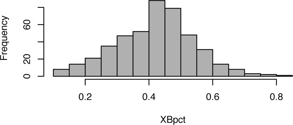
Here is the code for calculating the distribution of base running ratings in 2004. Figure 5-13 shows the histogram. Note that the distribution is roughly normal, with the average rating near 43%.

	hist(subset(XBRpct, EBR>19), main="", xlab="XBRpct", breaks=20)

Figure 5-13. Distribution of extra base running percentage

It would be great to fit these measurements into the linear weights system, and doing so is straightforward. From the expected runs matrix, we know how many runs are expected with runners on first and third (instead of first and second) after a single, to score from first after a double (as opposed to leaving a runner on third), and to score from second on a single (instead of holding at third). We can easily extrapolate the value of these moves in terms of runs.

Additionally, you can adjust these figures to account for differences between ballparks. I skipped this step to keep this hack simple. For information on calculating ballpark effects, see “Measure Park Effects” [Hack #56] .