CHAPTER 9
Understand the Regression Model
“Regression analysis is like one of those fancy power tools. It is relatively easy to use, but hard to use well—and potentially dangerous when used improperly.”
Charles Wheelan in Naked Statistics1
SUPERVISED LEARNING
The preceding chapter showcased unsupervised learning—discovering patterns or clusters in a dataset without predefined groups. Remember, in unsupervised learning, we come with no preconceived notions or patterns. We instead take advantage of the underlying aspects of data, establish some guardrails, and then let the data organize itself.
However, there will be many occasions when you do in fact know something about the underlying data. In that case, you'll need to use supervised learning to find relationships in data with inputs and known outputs. Here, you have the correct answers to “learn” from. You can then judge the robustness of the model against what you know about the real world. A good model will allow you to make accurate predictions and provide some explanation to the underlying relationships between the data's inputs and outputs.
Supervised learning, as you might recall, made an early cameo in the book's Introduction, back when you first started your Data Head journey. We asked you to predict if a new restaurant location would be a chain or independent restaurant. To make your guess, you first learned from existing restaurant locations (inputs) and known labels of “chain” or “independent” (outputs). You detected relationships between the inputs and outputs to create a “model” in your head that you used to make an educated prediction about the label for a new location.
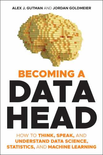
You might be surprised to learn all supervised learning problems follow that same paradigm, depicted in Figure 9.1. Data with inputs and outputs, called training data, is fed into an algorithm that exploits the relationships between the inputs and outputs to create a model (think equation) that makes predictions. The model can take a new input and map it to a predicted output. When the output is a number, the supervised learning model is called a regression model. When the output is a label (aka categorical variable), the model is called a classification model.
You'll learn about regression models now and classification models in the next chapter.
This paradigm encapsulates many exciting and practical supervised learning problems found in technologies both old and new. The spam detector in your email, your home or apartment's estimated value, speech translation, facial detection applications, and self-driving cars—these all use supervised learning. Table 9.1 breaks down some of these applications into their inputs, outputs, and model types.
As the applications of supervised learning have become more advanced, it's easy to lose sight that these applications are rooted in a classic method created around 1800 called linear regression. Linear regression, specifically least squares regression,2 is a workhorse in supervised learning and often the first approach your data workers will try when they want to make predictions. It's ubiquitous, powerful, and (don't be surprised) misused.
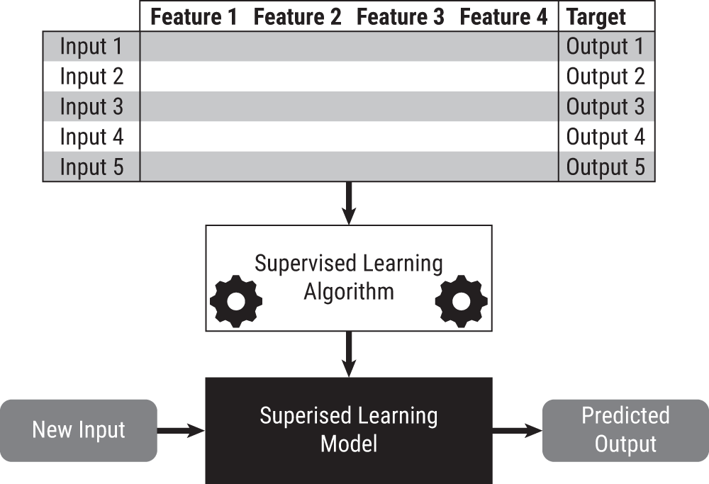
FIGURE 9.1 Basic paradigm of supervised learning: mapping inputs to outputs
TABLE 9.1 Applications of Supervised Learning
| Application | Input | Output | Model Type |
|---|---|---|---|
| Spam Detector | Email Text | Spam or Not Spam | Classification |
| Real Estate | Features and Location of House | Estimated Sales Price | Regression |
| Speech Translation | English Text | Chinese Text | Classification (each word is a label) |
| Facial Detection | Picture | Face Detected or No Face Detected | Classification |
| Smart Speakers | Audio | Did speaker hear “Alexa”? | Classification |
LINEAR REGRESSION: WHAT IT DOES
Suppose you run a small lemonade stand at the mall. You have a notion that temperature affects lemonade sales—specifically, the hotter it is outside, the more you'll sell. This prediction, if correct, could help you plan how much you'll need to buy and which days will sell more.
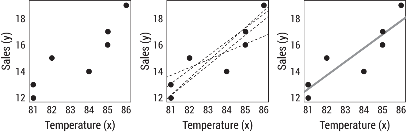
FIGURE 9.2 Many lines would fit this data reasonably well, but which line is the best? Linear regression will tell us.
You plot some historical data, the left plot in Figure 9.2, and spot what appears to be a nice linear trend. If you fit a line through this data, you could use the equation 3 Sales = m(Temperature) + b. A simple equation like this is a type of model.4 But how would you choose the numbers m (called the slope) and b (the intercept) to build your model?
Well, you could take a few stabs at it on your own. The center plot of Figure 9.2 shows four possible lines—these guesses all seem reasonable. But they're just guesses—they're not optimized to explain the underlying relationship given the data, even though they are close.
Linear regression employs a computational method to produce the line of best fit. By best fit, we mean that the line itself is optimized to explain as much linear trend and scatter of the data as possible. To the extent mathematically possible, it represents an optimal solution given the data provided. The rightmost chart in Figure 9.2 employs linear regression with the resultant equation: Sales = 1.03(Temperature) – 71.07.
Let's see how this works.
Least Squares Regression: Not Just a Clever Name
For a moment, let's just focus on our output variable—lemonade sales. If we wanted to figure out how much lemonade you might sell in the future, a reasonable prediction could be the mean of past sales (12 + 13 + 15 + 14 + 17 + 16 + 19) / 7 = $15.14. In short, we have an easy linear model, where Sales = $15.14.
Notice, this is still a linear equation, just without temperature. That means, no matter what the temperature is, we're going to predict sales of $15.14. We know it's naive, but it does fit our definition of a model that maps inputs to outputs, even if every output happens to be the same.
So how well does our simple model do? To measure the model's performance, let's calculate how far away the predicted sales value is from each of the actual sales. When the temperature was 86, sales were $19; the model predicted $15.14. When the temperature was 81, sales were $12; the model again predicted $15.14. The first instance represents an underprediction of about $4; the second, an overprediction of about $3. So far, we see that our model isn't perfect. And to really understand its ability to predict well, we'll need to understand the difference between what our model predicted and what actually happened. These differences are called errors—and they represent how far off our prediction is from what we know to be true.
So how could we measure these errors to understand how well our model is doing? Well, we could take every actual sales price and subtract it from the mean, which we predicted to be $15.14. But if you do this, you'll see that every error, when summed up, always totals to zero. That's because the mean, which we're using as our predictor, represents the arithmetic center of these points. Subtracting the difference of all these points to the center makes the result zero.
But we do need a way to aggregate these errors because, clearly, the model isn't perfect. The most common approach is called the least squares method. And, in this approach, we instead square the differences from our prediction to make everything positive.5 When we add up these numbers, the result won't be zero (unless, in fact, there is no error in our data). We call the result the sum of squares.
Let's take a look at Figure 9.3(a). You'll see the original scatter plot with x = Temperature and y = Sales. Notice, we've applied our naive model: temperature has no effect on the prediction. That is, the prediction is always 15.14, which gives a horizontal line at Sales = 15.14. In other words: the data point with temperature = 86 and actual sales = 19 has predicted sales of 15.14. The solid vertical line shows the difference between the actual value and predicted value for this point (and all other points). In regression, you square these lengths to create a square with area 14.9.
When sales were $15, our model still predicted $15.14, thus the corresponding square has an area of (15.14 – 15)2 = 0.02. Add up the areas (sum the squares) from all points to represent the total error of your simple model. The squares you see on the right plot of Figure 9.3(a) are a visual representation of the squared error calculations. The larger the sum of squares, the worse the model fits the data. The smaller the sum of squares, the better the fit.
The question then becomes, can we arrive at a slope and intercept that would optimize (that is, reduce) the sum of squared errors as much as possible? Right now, our naive model has no slope, but it does have an intercept of $15.14.
Clearly 9.3(a) doesn't do the best job. To get even closer to a good fit, let's add a slope m, which brings temperature into the equation. In Figure 9.3(b), we speculate a reasonable slope and intercept could be 0.6 and –34.91, respectively. Notice that adding this relationship makes our flat-lined model from 9.3(a) into a sloped line that appears to capture some upward trend. You can also immediately see a reduction in the overall area of the squares.
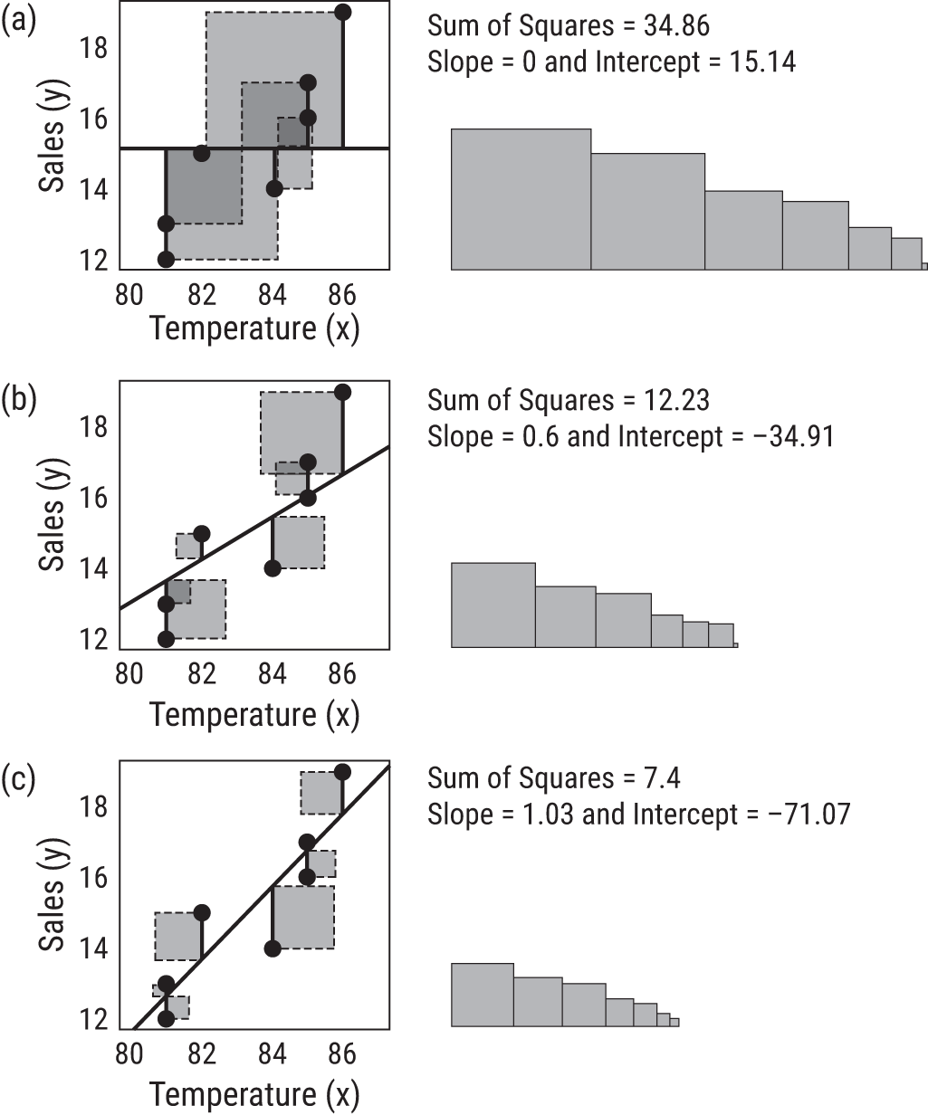
FIGURE 9.3 Least squares regression is finding the line through the data that results in the least squares (in terms of area) of the predicted values and the actual values.
Visually, the error has decreased substantially now that your model includes temperature. Your prediction for the point with temperature = 86 went from 15.14 in the simple model to Sales = 0.6(86) – 34.91= 16.69, which reduced this observation's contribution to the sum of squares from 14.9 to (16.69 – 19)2 = 5.34.
You could do the guesswork yourself—that is, plugging numbers into the slope and intercept until you might get the one combination that would reduce the sum of squares to its mathematical minimum. But linear regression does this for you mathematically. Figure 9.3(c) shows, quite literally, the least amount of squared errors you can see with this data. The slightest derivation from these slope and intercept numbers would make those squares bigger.
You can use the information to assess how well the final model fits the data. Note Figure 9.3(c), which contains the linear regression result, is still imperfect. But you can clearly see it's better than Figure 9.3(a) where you predicted $15.14 each time.
How much better? Well, you started with an area (sum of squares) of 34.86, and the final model reduced the area to 7.4. That means we've reduced the area of the control model by (34.86 – 7.4) = 27.46, which is a 27.46/34.86 = 78.8% percent reduction in total area. You'll often hear people say the model has “explained,” “described,” or “predicted” 78.8% (or 0.788) of the variation in the data. This number is called “R-squared” or R2.
If the model fits the data perfectly, R2 = 1. But don't count on seeing such models with a high R2 in your work.6 If you do, someone probably made a mistake—and you should ask to review the data collection processes. Recall from Chapter 3 that variation is in everything, and there's always variation we can't fully explain. That's just how the universe is.
LINEAR REGRESSION: WHAT IT GIVES YOU
Let's quickly review what we've discussed and tie this back to the supervised learning paradigm in Figure 9.1. You had a dataset with one input column and one output column that was fed into the linear regression algorithm. The algorithm learned from the data the best numbers to finalize the linear equation Sales = m(Temperature) + b and produced the model Sales = 1.03(Temperature) – 71.07 that you can use to make predictions about how much money you'll make selling lemonade.
Linear regression models are favorites in many industries because they not only make predictions, but also offer explanations about how the input features relate to the output. (Also, they're not hard to compute.) The slope coefficient, 1.03, tells you for every one unit increase in temperature, you can expect sales to increase by $1.03. This number provides both a magnitude and direction for the impact of the input on the output.
Recognizing there is randomness and variability in the world and the data we capture from it, you can imagine that the coefficient numbers from linear regression have some variability built in. If you collected a new set of data from your lemonade stand, perhaps the impact from temperature would change from $1.03 to $1.25. The data fed into the algorithm is a sample, and thus you must continue to think statistically about the results. Statistical software helps you do this by outputting p-values for each coefficient (testing the null hypothesis, H0: the coefficient = 0), letting you know if the coefficient is statistically different than zero. For instance, a coefficient of 0.000003 is very close to zero, and might reflect something that for practical purposes is a zero in your model.
Put differently, if the coefficient is not statistically different than zero, you can drop that feature from your model. The input is not impacting the output, so why include it? Of course, statistics lessons from Chapter 6 remain relevant. A coefficient may indeed be statistically significant but not practically so. Always ask to see the coefficients of models impacting your business.
Extending to Many Features
Your business, we assume, is a little more complicated than a lemonade stand. Your sales would not only be a function of temperature (if a seasonal business), but many other features or inputs. Fortunately, the simple linear regression model you've learned about can be extended to include many features.7 Regression with one input is called simple linear regression; with multiple inputs, it's called multiple linear regression.
To show you an example, we fit a quick multiple linear regression line to the housing data we explored in Chapter 5. This data had 1234 houses and 81 inputs, but to simplify the example, we're going to look at 6 inputs. (We could have also used PCA to reduce the dimensionality, but we didn't want to overcomplicate this example.)
TABLE 9.2 Multiple Linear Regression Model Fit to Housing Data. All corresponding p-values are statistically significant at the 0.05 significance level.
| Input | Coefficient | p-value |
|---|---|---|
| (Intercept) | –1614841.60 | <0.000 |
| LotArea | 0.54 | <0.000 |
| YearBuilt | 818.38 | <0.000 |
| 1stFlrSF | 87.43 | <0.000 |
| 2ndFlrSF | 90.00 | <0.000 |
| TotalBsmtSF | 53.24 | <0.000 |
| FullBath | –7398.13 | 0.017 |
Let's build a model to predict the sales price of a home (output) based on lot area, year built, 1st floor square footage, 2nd floor square footage, basement square footage, and number of full bathrooms. The linear regression algorithm will work its magic, learn from the data, and output the best coefficients to complete the model, resulting in the intercept and coefficients in Table 9.2.
A core tenet of a multiple regression model is to isolate the effect of one variable while controlling for the others. We can say, for example, if all other inputs are held constant, a home built one year sooner adds (on average) $818.38 to the sales price. The coefficients of each feature are showing the magnitude and direction the input has on price. Make sure to consider the units. Adding 1 unit to square footage is different than adding 1 unit to the number of bathrooms. A statistician can scale these appropriately if you need an apples-to-apples comparison between coefficients.
Each coefficient also undergoes an associated statistical test to let us know if it's statistically different than zero. If it is not, we can safely remove it from the model because it doesn't add information or change the output.
LINEAR REGRESSION: WHAT CONFUSION IT CAUSES
If your esteemed authors were con men, we would have ended the chapter with the previous section and asked you to purchase linear regression software as the cure-all for your business needs. Our sales pitch would be “Enter data, get a model, and start making predictions about your business today!” That sounds fantastically easy, but by this point you've gotten to know data well enough that nothing is as easy at seems (or as easy as it's sold). Like the quote we used to start the chapter, linear regression in the wrong hands can be potentially dangerous. So whether you create or use regression models, always maintain a healthy skepticism. The equations, terminology, and computation make it seem like a linear regression model can autocorrect any issue in your dataset. It can't.
Let's go through some of the pitfalls of using linear regression.
Omitted Variables
Supervised learning models cannot learn the relationship between an input variable and an output variable if the input variable was omitted from the model. Consider our simple model that predicted lemonade sales based on average past sales but without regard to temperature.
Data Heads like yourself, now aware of this issue, might suggest informative, relevant features to include in models. But don't just leave feature selection up to your data workers. Subject matter expertise and getting the right data into a supervised learning model is key to having a successful model.
For example, the housing model in the previous section has an R2 value of 0.75. This means we've explained 75% of the variation in sales price with our model. Now think about features not in this model that would help one predict a home's price—perhaps things like economic conditions, interest rates, elementary school ratings, etc. These omitted variables not only impact predictions of the model but may lead to dubious interpretations. Did you notice in Table 9.2 the coefficient for the number of bathrooms was negative? That doesn't make sense.
Here's another example. Consider a linear regression model that “learned” shoe size has a large positive coefficient in a linear regression model for the number of words a person can read per minute. Age is clearly a missing input variable here: including it would remove the need for “shoe size” as an input. Certainly, examples in your work may not be as easy to tease out as this example but believe us when we say omitted variables can and will cause headaches and misinterpretations. Further, many things are correlated with time, a common omitted variable.
We hope the phrase “correlation does not mean causation” comes to mind once again while reading this section. Having one variable labeled as an input to a model and another as an output does not mean the input causes the output.
Multicollinearity
If your goal with linear regression is interpretability—to be able to study the impact of the input variables on the output by studying the coefficients—then you must be aware of multicollinearity. This means several variables are correlated, and it creates a direct challenge to your model being interpretable.
Recall, a goal of multiple regression is to isolate the effect of one input's contribution while holding every other input constant. But this is only possible if the underlying data is uncorrelated.
To offer a quick example, suppose the lemonade stand data we plotted earlier had the temperature in both Celsius and Fahrenheit. Obviously, the two are perfectly correlated because one is a function of the other, but for this example, suppose each temperature reading was taken with a different instrument to introduce some variation.8 The model would go from:
- Sales = 1.03(Temperature) – 71.07 to
- Sales = –0.2(Temperature in F) + 2.1(Temperature in C) – 30.8.
Now it looks like adding a degree in Fahrenheit has a negative impact! Yet, we know the inputs are comingled—in fact, redundant—and linear regression cannot break apart the relationship. Multicollinearity is present in most observational datasets, so consider this a fair warning. Data collected experimentally, however, is specifically designed to prevent the inputs from being multicollinear to the extent possible.9
Data Leakage
Imagine building a model to predict the sales price of a home (like we did earlier in the chapter). But this time, the training data not only includes features about the home (size, number of bedrooms, etc.), but also the initial offer made on the house. A snapshot of the dataset is shown in Table 9.3.
If you run the model on the data, you might notice that the initial offer is very predictive of the sales price. Great!—you think. You can rely on that to help you predict home prices for your company.
The model then goes into production. You attempt to run the model only to find that you don't have access to the initial offer on the houses whose sales prices you are trying to predict—they haven't sold yet! This is an example of data leakage. Data leakage10 happens when a concurrent output variable masquerades as an input variable.
The problem with using the initial offer is one of timing. Consider for a moment that you could only learn what the starting offer was after the home was already sold.
As we are immersed in data, data leakage is easy to overlook. Sadly, many textbooks don't cover it because the datasets inside are pristine for learning, but real-world datasets always have the possibility for leakage. As a Data Head, you must be on the lookout to ensure your input and output data do not contain overlapping information.
We will explore data leakage again in later chapters.
TABLE 9.3 Sample Housing Data
| Square Footage | Bedrooms | Baths | Initial Offer | Sales Price |
|---|---|---|---|---|
| 1500 | 2 | 1 | $190,000 | $200,000 |
| 2000 | 3 | 2 | $240,000 | $250,000 |
| 2500 | 4 | 3 | $300,000 | $300,000 |
Extrapolation Failures
Extrapolation means predicting beyond the range of the input data you used to build your model. If the temperature was 00F, the lemonade stand model would predict sales of –$71.07. If a house had no square footage and no bathrooms (practically speaking, the house wouldn't exist), the model would predict a sales price of –$1,614,841.60. Both cases are nonsense.
The models are predicting outside the range of data they “learned” from, and unlike humans, equations don't have common sense to know it's wrong. Math equations cannot think. If you give it numbers as inputs, it will spit back a number as an output. It's up to you, the Data Head, to know if extrapolation is taking place.
It must be stressed that model results are always predicted on the given data. Which is to say, you should not make predictions with data that “fits” the range of the training data but not the context in which the dataset was collected. The model has no context for changes taking place in the world.
If you built a model that predicted housing prices in 2007, your model would have performed terribly in 2008 after the housing market crashed. Using the model in 2008 would have extrapolated the market conditions of 2007 data to be vastly different in 2008. Industries are facing this at the time of writing, 2021, because of the COVID-19 pandemic. Models trained on pre-COVID data no longer reflect many of the relationships identified, and the models are no longer valid.
Many Relationships Aren't Linear
Linear regression would not do well modeling the performance of the stock market. Historically, it has grown exponentially, not linearly. The Statistics department at Procter & Gamble would offer this advice: “Don't fit a straight line through a banana.”
Statisticians have tools in their arsenal to transform some non-linear data into linear data. Even so, sometimes, you must accept that linear regression is not the right tool for the job.
Are You Explaining or Predicting?
Throughout this chapter, we've been discussing two possible goals with regression models: explain relationships and make predictions. Linear regression models can seemingly do both. A linear regression model's coefficients (under the right conditions) offer interpretability. Many industries focus their attention on interpretability—like in clinical trials where researchers need to know the precise magnitude and direction of the input “dosage of a medicine” to the output “blood pressure.” In this case, great care must be taken to avoid multicollinearity and omitted variables to ensure model explanations are possible.
In other fields, like machine learning, accurate prediction is the goal.11 The presence of multicollinearity, for example, may not be a concern if the model can predict future outputs well. When the purpose of a model is to predict new outputs, you absolutely must be careful to avoid overfitting the data.
Recall that models are simplified versions of reality. A good model approximates the relationships between inputs and outputs well. Indeed, it's capturing some underlying phenomenon. The data itself is merely an expression of this underlying phenomenon.
An overfit model, however, does not capture that relationship we speculate exists. Rather it captures the interaction of the training data, including the noise and variation in the data itself. Thus, the predictions it makes are not what's being modeled, but rather just the data points we have.
Models that overfit effectively memorize the sample training data. They don't generalize well to new observations. Check out Figure 9.4. On the left, you see the lemonade data with the linear regression model. On the right, a complex regression model that perfectly predicts some of the points. Which would you want to use to make a prediction?
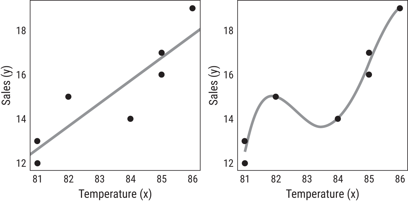
FIGURE 9.4 Two competing models. The model on the left generalizes well, while the model on the right overfits the data, effectively memorizing the data. Because of variation, the model on the right will not predict new points well.
The way to prevent overfitting is to split a dataset into two parts: a training set you use to build a model and a test set to see how it performs. The performance on your test set, data your model did not learn from, will be the ultimate judge of how well your model predicts.
Regression Performance
Whenever you come across a regression model at work, whether it's a multiple linear regression model or something more sophisticated that was just invented last week, the best way to judge how well it fits your data is with an “actual by predicted” plot. In our experience, some people assume we can't visualize regression performance when we have too many inputs, but remember what the model has done. It converted inputs (either one or several) into an output.
So, for each row in your dataset, you have the actual value and its associated predicted value. Plot them in a scatter plot! These should be well correlated. This eye-ball test will let you know quickly how well your model has done. Your data workers can provide several associated metrics (R-squared being one), but never look at those numbers alone. Always, always demand to see the actual vs. predicted plot. An example is shown in Figure 9.5 using the model we built on the housing data.
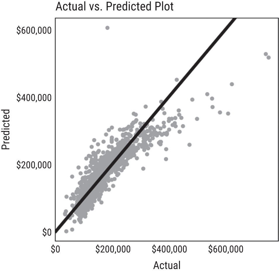
FIGURE 9.5 In this plot, you can see how the model does not do well predicting high-value homes. Can you spot other issues with this model using this chart?
OTHER REGRESSION MODELS
Finally, you may come across some variants of linear regression called LASSO and Ridge Regression that help when there are many correlated inputs (multicollinearity) or when you have more input variables than rows in your dataset. The result is a model that looks similar to multiple regression models.
Other regression models look completely different. K-nearest neighbor from the Introduction was applied to a classification problem, but it can easily be applied to a regression problem. For instance, to predict the sales price of any home, we could take the mean selling price of the three closest homes to it that recently sold. This would use K-nearest neighbor as a regression problem.
We'll go over some of these models in the next chapter, as they can be used for both regression or classification.
CHAPTER SUMMARY
Our goal was to help you develop an intuitive understanding of supervised learning and its most fundamental algorithm, linear regression. We then examined the many ways regression models can go wrong. Keep those issues and pitfalls in your mind because it's not a matter of which will impact regression models in your workplace, but how many.
As you might have put together by now, supervised learning is both powered and limited by the training data. Unfortunately, we see companies spending more time worried about the latest supervised learning algorithm rather than thinking about how to collect relevant, accurate, and enough data to feed the algorithm. Please, do not forget about the “garbage in, garbage out” mantra from earlier in the book. Good data is key and is the lifeforce for supervised learning models.
And at this point, we can reveal that if you understood unsupervised learning and supervised learning, you now understand machine learning. Congrats! And apologies for the lack of a big reveal. We wanted to be the antithesis of a sales pitch and teach you components of machine learning without getting bogged down by hype. Machine learning is unsupervised learning and supervised learning.
Let's continue this conversation about machine learning in the next chapter with classification models.
NOTES
- 1 Wheelan, C. (2013). Naked statistics: Stripping the dread from the data. WW Norton & Company.
- 2 It's usually safe to assume “least squares regression” whenever you hear “linear regression,” unless stated otherwise. There are other types of linear regression, but least squares is the most popular.
- 3 In Algebra, you learned the equation of a line: y = mx + b. For any input x, you can get an output y by multiplying x and m and adding b. If y = 2x + 5, then an input x = 7 gives the output y = 2×7 + 5 = 19.
- 4 Quick terminology reminder: the output y is called the target, response variable, or dependent variable. The input x is called a feature, predictor, or independent variable. You may hear all terms in your work.
- 5 Taking the absolute values would also make the errors positive before aggregating. However, squaring has nicer mathematical properties than the absolute value in that it is differentiable—this was vital to the early uses of linear regression because they had to do this all by hand.
- 6 For simple regression with one input, R2 is the square of the correlation coefficient we discussed in Chapter 5. It is possible, however, for R2 to be negative. This happens when the linear regression model is worse than predicting the mean.
- 7 The upper limit for the number of features/inputs in a linear regression model is N – 1, where N is the number of rows in your dataset. Thus, you can have up to 11 inputs to predict monthly sales for a 12-month period.
- 8 Linear regression models will not compute if two inputs are perfectly correlated, so we added noise to this example.
- 9 There is an entire field of Statistics called Design of Experiments devoted to this idea.
- 10 en.wikipedia.org/wiki/Leakage_(machine_learning)
- 11 There's a great paper that goes into depth about the difference between explaining and prediction for models: Shmueli, G. (2010). To explain or to predict? Statistical science, 25(3), 289–310.