
![]()
Spark Core
Spark is the most active open source project in the big data world. It has become hotter than Hadoop. It is considered the successor to Hadoop MapReduce, which we discussed in Chapter 1. Spark adoption is growing rapidly. Many organizations are replacing MapReduce with Spark.
Conceptually, Spark looks similar to Hadoop MapReduce; both are designed for processing big data. They both enable cost-effective data processing at scale using commodity hardware. However, Spark offers many advantages over Hadoop MapReduce. These are discussed in detail later in this chapter.
This chapter covers Spark core, which forms the foundation of the Spark ecosystem. It starts with an overview of Spark core, followed by the high-level architecture and runtime view of an application running on Spark. The chapter also discusses Spark core’s programming interface.
Overview
Spark is an in-memory cluster computing framework for processing and analyzing large amounts of data. It provides a simple programming interface, which enables an application developer to easily use the CPU, memory, and storage resources across a cluster of servers for processing large datasets.
Key Features
The key features of Spark include the following:
Easy to Use
Spark provides a simpler programming model than that provided by MapReduce. Developing a distributed data processing application with Spark is a lot easier than developing the same application with MapReduce.
Spark offers a rich application programming interface (API) for developing big data applications; it comes with 80-plus data processing operators. Thus, Spark provides a more expressive API than that offered by Hadoop MapReduce, which provides just two operators: map and reduce. Hadoop MapReduce requires every problem to be broken down into a sequence of map and reduce jobs. It is hard to express non-trivial algorithms with just map and reduce. The operators provided by Spark make it easier to do complex data processing in Spark than in Hadoop MapReduce.
In addition, Spark enables you to write more concise code compared to Hadoop MapReduce, which requires a lot of boilerplate code. A data processing algorithm that requires 50 lines of code in Hadoop MapReduce can be implemented in less than 10 lines of code in Spark. The combination of a rich expressive API and the elimination of boilerplate code significantly increases developer productivity. A developer can be five to ten times more productive with Spark as compared to MapReduce.
Fast
Spark is orders of magnitude faster than Hadoop MapReduce. It can be hundreds of times faster than Hadoop MapReduce if data fits in memory. Even if data does not fit in memory, Spark can be up to ten times faster than Hadoop MapReduce.
Speed is important, especially when processing large datasets. If a data processing job takes days or hours, it slows down decision-making. It reduces the value of data. If the same processing can be run 10 to 100 times faster, it opens the door to many new opportunities. It becomes possible to develop new data-driven applications that were not possible before.
Spark is faster than Hadoop MapReduce for two reasons. First, it allows in-memory cluster computing. Second, it implements an advanced execution engine.
Spark’s in-memory cluster computing capabilities provides an orders of magnitude performance boost. The sequential read throughput when reading data from memory compared to reading data from a hard disk is 100 times greater. In other words, data can be read from memory 100 times faster than from disk. The difference in read speed between disk and memory may not be noticeable when an application reads and processes a small dataset. However, when an application reads and processes terabytes of data, I/O latency (the time it takes to load data from disk to memory) becomes a significant contributor to overall job execution time.
Spark allows an application to cache data in memory for processing. This enables an application to minimize disk I/O. A MapReduce-based data processing pipeline may consist of a sequence of jobs, where each job reads data from disk, processes it, and writes the results to disk. Thus, a complex data processing application implemented with MapReduce may read data from and write data to disk several times. Since Spark allows caching of data in memory, the same application implemented with Spark reads data from disk only once. Once data is cached in memory, each subsequent operation can be performed directly on the cached data. Thus, Spark enables an application to minimize I/O latency, which, as previously mentioned, can be a significant contributor to overall job execution time.
Note that Spark does not automatically cache input data in memory. A common misconception is that Spark cannot be used if input data does not fit in memory. It is not true. Spark can process terabytes of data on a cluster that may have only 100 GB total cluster memory. It is up to an application to decide what data should be cached and at what point in a data processing pipeline that data should be cached. In fact, if a data processing application makes only a single pass over data, it need not cache data at all.
The second reason Spark is faster than Hadoop MapReduce is that it has an advanced job execution engine. Both Spark and MapReduce convert a job into a directed acyclic graph (DAG) of stages. In case you are not familiar with graph theory, a graph is a collection of vertices connected by edges. A directed graph is a graph with edges that have a direction. An acyclic graph is a graph with no graph cycles. Thus, a DAG is a directed graph with no directed cycles. In other words, there is no way you can start at some vertex in a DAG and follow a sequence of directed edges to get back to the same vertex. Chapter 11 provides a more detailed introduction to graphs.
Hadoop MapReduce creates a DAG with exactly two predefined stages—Map and Reduce—for every job. A complex data processing algorithm implemented with MapReduce may need to be split into multiple jobs, which are executed in sequence. This design prevents Hadoop MapReduce from doing any optimization.
In contrast, Spark does not force a developer to split a complex data processing algorithm into multiple jobs. A DAG in Spark can contain any number of stages. A simple job may have just one stage, whereas a complex job may consist of several stages. This allows Spark to do optimizations that are not possible with MapReduce. Spark executes a multi-stage complex job in a single run. Since it has knowledge of all the stages, it optimizes them. For example, it minimizes disk I/O and data shuffles, which involves data movement across a network and increases application execution time.
General Purpose
Spark provides a unified integrated platform for different types of data processing jobs. It can be used for batch processing, interactive analysis, stream processing, machine learning, and graph computing. In contrast, Hadoop MapReduce is designed just for batch processing. Therefore, a developer using MapReduce has to use different frameworks for stream processing and graph computing.
Using different frameworks for different types of data processing jobs creates many challenges. First, a developer has to learn multiple frameworks, each of which has a different interface. This reduces developer productivity. Second, each framework may operate in a silo. Therefore, data may have to be copied to multiple places. Similarly, code may need to be duplicated at multiple places. For example, if you want to process historical data with MapReduce and streaming data with Storm (a stream-processing framework) exactly the same way, you have to maintain two copies of the same code—one in Hadoop MapReduce and the other in Storm. The third problem with using multiple frameworks is that it creates operational headaches. You need to set up and manage a separate cluster for each framework. It is more difficult to manage multiple clusters than a single cluster.
Spark comes pre-packaged with an integrated set of libraries for batch processing, interactive analysis, stream processing, machine learning, and graph computing. With Spark, you can use a single framework to build a data processing pipeline that involves different types of data processing tasks. There is no need to learn multiple frameworks or deploy separate clusters for different types of data processing jobs. Thus, Spark helps reduce operational complexity and avoids code as well as data duplication.
Interestingly, many popular applications and libraries that initially used MapReduce as an execution engine are either being migrated to or adding support for Spark. For example, Apache Mahout, a machine-learning library initially built on top of Hadoop MapReduce, is migrating to Spark. In April 2014, the Mahout developers said goodbye to MapReduce and stopped accepting new MapReduce-based machine learning algorithms.
Similarly, the developers of Hive (discussed in Chapter 1) are developing a version that runs on Spark. Pig, which provides a scripting language for building data processing pipelines, has also added support for Spark as an execution engine. Cascading, an application development platform for building data applications on Hadoop, is also adding support for Spark.
Scalable
Spark is scalable. The data processing capacity of a Spark cluster can be increased by just adding more nodes to a cluster. You can start with a small cluster, and as your dataset grows, you can add more computing capacity. Thus, Spark allows you to scale economically.
In addition, Spark makes this feature automatically available to an application. No code change is required when you add a node to a Spark cluster.
Fault Tolerant
Spark is fault tolerant. In a cluster of a few hundred nodes, the probability of a node failing on any given day is high. The hard disk may crash or some other hardware problem may make a node unusable. Spark automatically handles the failure of a node in a cluster. Failure of a node may degrade performance, but will not crash an application.
Since Spark automatically handles node failures, an application developer does not have to handle such failures in his application. It simplifies application code.
Ideal Applications
As discussed in the previous section, Spark is a general-purpose framework; it can be used for a variety of big data applications. However, it is ideal for big data applications where speed is very important. Two examples of such applications are applications that allow interactive analysis and applications that use iterative data processing algorithms.
Iterative Algorithms
Iterative algorithms are data processing algorithms that iterate over the same data multiple times. Applications that use iterative algorithms include machine learning and graph processing applications. These applications run tens or hundreds of iterations of some algorithm over the same data. Spark is ideal for such applications.
The reason iterative algorithms run fast on Spark is its in-memory computing capabilities. Since Spark allows an application to cache data in memory, an iterative algorithm, even if it runs 100 iterations, needs to read data from disk only for the first iteration. Subsequent iterations read data from memory. Since reading data from memory is 100 times faster than reading from disk, such applications run orders of magnitude faster on Spark.
Interactive Analysis
Interactive data analysis involves exploring a dataset interactively. For example, it is useful to do a summary analysis on a very large dataset before firing up a long-running batch processing job that may run for hours. Similarly, a business analyst may want to interactively analyze data using a BI or data visualization tool. In such cases, a user runs multiple queries on the same data. Spark provides an ideal platform for interactively analyzing a large dataset.
The reason Spark is ideal for interactive analysis is, again, its in-memory computing capabilities. An application can cache the data that will be interactively analyzed in memory. The first query reads data from disk, but subsequent queries read the cached data from memory. Queries on data in memory execute orders of magnitude faster than on data on disk. A query that takes more than an hour when it reads data from disk may take seconds when it is run on the same data cached in memory.
High-level Architecture
A Spark application involves five key entities: a driver program, a cluster manager, workers, executors, and tasks (see Figure 3-1).
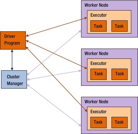
Figure 3-1. High-level Spark architecture
Workers
A worker provides CPU, memory, and storage resources to a Spark application. The workers run a Spark application as distributed processes on a cluster of nodes.
Cluster Managers
Spark uses a cluster manager to acquire cluster resources for executing a job. A cluster manager, as the name implies, manages computing resources across a cluster of worker nodes. It provides low-level scheduling of cluster resources across applications. It enables multiple applications to share cluster resources and run on the same worker nodes.
Spark currently supports three cluster managers: standalone, Mesos, and YARN. Mesos and YARN allow you to run Spark and Hadoop applications simultaneously on the same worker nodes. These cluster managers are discussed in more detail in Chapter 10.
Driver Programs
A driver program is an application that uses Spark as a library. It provides the data processing code that Spark executes on the worker nodes. A driver program can launch one or more jobs on a Spark cluster.
Executors
An executor is a JVM (Java virtual machine) process that Spark creates on each worker for an application. It executes application code concurrently in multiple threads. It can also cache data in memory or disk.
An executor has the same lifespan as the application for which it is created. When a Spark application terminates, all the executors created for it also terminate.
Tasks
A task is the smallest unit of work that Spark sends to an executor. It is executed by a thread in an executor on a worker node. Each task performs some computations to either return a result to a driver program or partition its output for shuffle.
Spark creates a task per data partition. An executor runs one or more tasks concurrently. The amount of parallelism is determined by the number of partitions. More partitions mean more tasks processing data in parallel.
Application Execution
This section briefly describes how data processing code is executed on a Spark cluster.
Terminology
Let’s define a few terms first:
- Shuffle. A shuffle redistributes data among a cluster of nodes. It is an expensive operation because it involves moving data across a network. Note that a shuffle does not randomly redistribute data; it groups data elements into buckets based on some criteria. Each bucket forms a new partition.
- Job. A job is a set of computations that Spark performs to return results to a driver program. Essentially, it is an execution of a data processing algorithm on a Spark cluster. An application can launch multiple jobs. Exactly how a job is executed is covered later in this chapter.
- Stage. A stage is a collection of tasks. Spark splits a job into a DAG of stages. A stage may depend on another stage. For example, a job may be split into two stages, stage 0 and stage 1, where stage 1 cannot begin until stage 0 is completed. Spark groups tasks into stages using shuffle boundaries. Tasks that do not require a shuffle are grouped into the same stage. A task that requires its input data to be shuffled begins a new stage.
How an Application Works
With the definitions out of the way, I can now describe how a Spark application processes data in parallel across a cluster of nodes. When a Spark application is run, Spark connects to a cluster manager and acquires executors on the worker nodes. As mentioned earlier, a Spark application submits a data processing algorithm as a job. Spark splits a job into a directed acyclic graph (DAG) of stages. It then schedules the execution of these stages on the executors using a low-level scheduler provided by a cluster manager. The executors run the tasks submitted by Spark in parallel.
Every Spark application gets its own set of executors on the worker nodes. This design provides a few benefits. First, tasks from different applications are isolated from each other since they run in different JVM processes. A misbehaving task from one application cannot crash another Spark application. Second, scheduling of tasks becomes easier. Spark has to schedule the tasks belonging to only one application at a time. It does not have to handle the complexities of scheduling tasks from multiple concurrently running applications.
However, this design also has one disadvantage. Since applications run in separate JVM processes, they cannot easily share data. Even though they may be running on the same worker nodes, they cannot share data without writing it to disk. As previously mentioned, writing and reading data from disk are expensive operations. Therefore, applications sharing data through disk will experience performance issues.
Data Sources
Spark is essentially a computing framework for processing large datasets using a cluster of nodes. Unlike a database, it does not provide a storage system, but it works in conjunction with external storage systems. Generally, it is used with distributed storage systems that store large amounts of data.
Spark supports a variety of data sources. The data that you crunch through a Spark application can be in HDFS, HBase, Cassandra, Amazon S3, or any other Hadoop-supported data source. Any data source that works with Hadoop can be used with Spark core. One of the Spark libraries, Spark SQL, enables Spark to support even more data sources. Chapter 7 covers Spark SQL.
Compatibility with a Hadoop-supported data source is important. Organizations have made significant investments in Hadoop. Large amounts of data exist in HDFS and other Hadoop-supported storage systems. Spark does not require you to move or copy data from these sources to another storage system. Thus, migration from Hadoop MapReduce to Spark is not a forklift operation. This makes it easy to switch from Hadoop MapReduce to Spark. If you have an existing Hadoop cluster running MapReduce jobs, you can run Spark applications on the same cluster in parallel. You can convert existing MapReduce jobs to Spark jobs. Alternatively, if you are happy with the existing MapReduce applications and do not want to touch them, you can use Spark for new applications.
While Spark core has built-in support for Hadoop compatible storage systems, support for additional data sources can be easily added. For example, people have created Spark connectors for Cassandra, MongoDB, CouchDB, and other popular data sources.
Spark also supports local file systems. A Spark application can read input from and store output to a local file system. Although Spark is not needed if data can be read from a local file and processed on a single computer, this capability is useful for initial application development and debugging. It also makes it easy to learn Spark.
Application Programming Interface (API)
Spark makes its cluster computing capabilities available to an application in the form of a library. This library is written in Scala, but it provides an application programming interface (API) in multiple languages. At the time this book is being written, the Spark API is available in Scala, Java, Python, and R. You can develop a Spark application in any of these languages. Unofficial support for additional languages, such as Clojure, is also available.
The Spark API consists of two important abstractions: SparkContext and Resilient Distributed Datasets (RDDs). An application interacts with Spark using these two abstractions. These abstractions allow an application to connect to a Spark cluster and use the cluster resources. The next section discusses each abstraction and then looks at RDDs in more detail.
SparkContext
SparkContext is a class defined in the Spark library. It is the main entry point into the Spark library. It represents a connection to a Spark cluster. It is also required to create other important objects provided by the Spark API.
A Spark application must create an instance of the SparkContext class. Currently, an application can have only one active instance of SparkContext. To create another instance, it must first stop the active instance.
The SparkContext class provides multiple constructors. The simplest one does not take any arguments. An instance of the SparkContext class can be created as shown next.
val sc = new SparkContext()
In this case, SparkContext gets configuration settings such as the address of the Spark master, application name, and other settings from system properties. You can also provide configuration parameters to SparkContext programmatically using an instance of SparkConf, which is also a class defined in the Spark library. It can be used to set various Spark configuration parameters as shown next.
val config = new SparkConf().setMaster("spark://host:port").setAppName("big app")
val sc = new SparkContext(config)
In addition to providing explicit methods for configuring commonly used parameters such as the address of the Spark master, SparkConf provides a generic method for setting any parameter using a key-value pair. The input parameters that you can provide to SparkContext and SparkConf are covered in more detail in Chapter 4.
The variable sc created earlier is used in other examples in the rest of this chapter.
Resilient Distributed Datasets (RDD)
RDD represents a collection of partitioned data elements that can be operated on in parallel. It is the primary data abstraction mechanism in Spark. It is defined as an abstract class in the Spark library.
Conceptually, RDD is similar to a Scala collection, except that it represents a distributed dataset and it supports lazy operations. Lazy operations are discussed in detail later in this chapter.
The key characteristics of an RDD are briefly described in the following sections.
Immutable
An RDD is an immutable data structure. Once created, it cannot be modified in-place. Basically, an operation that modifies an RDD returns a new RDD.
Partitioned
Data represented by an RDD is split into partitions. These partitions are generally distributed across a cluster of nodes. However, when Spark is running on a single machine, all the partitions are on that machine.
Note that there is a mapping from RDD partitions to physical partitions of a dataset. RDD provides an abstraction for data stored in distributed data sources, which generally partition data and distribute it across a cluster of nodes. For example, HDFS stores data in partitions or blocks, which are distributed across a cluster of computers. By default, there is one-to-one mapping between an RDD partition and a HDFS file partition. Other distributed data sources, such as Cassandra, also partition and distribute data across a cluster of nodes. However, multiple Cassandra partitions are mapped to a single RDD partition.
Fault Tolerant
RDD is designed to be fault tolerant. An RDD represents data distributed across a cluster of nodes and a node can fail. As previously discussed, the probability of a node failing is proportional to the number of nodes in a cluster. The larger a cluster, the higher the probability that some node will fail on any given day.
RDD automatically handles node failures. When a node fails, and partitions stored on that node become inaccessible, Spark reconstructs the lost RDD partitions on another node. Spark stores lineage information for each RDD. Using this lineage information, it can recover parts of an RDD or even an entire RDD in the event of node failures.
Interface
It is important to remember that RDD is an interface for processing data. It is defined as an abstract class in the Spark library. RDD provides a uniform interface for processing data from a variety of data sources, such as HDFS, HBase, Cassandra, and others. The same interface can also be used to process data stored in memory across a cluster of nodes.
Spark provides concrete implementation classes for representing different data sources. Examples of concrete RDD implementation classes include HadoopRDD, ParallelCollectionRDD, JdbcRDD, and CassandraRDD. They all support the base RDD interface.
Strongly Typed
The RDD class definition has a type parameter. This allows an RDD to represent data of different types. It is a distributed collection of homogenous elements, which can be of type Integer, Long, Float, String, or a custom type defined by an application developer. Thus, an application always works with an RDD of some type. It can be an RDD of Integer, Long, Float, Double, String, or a custom type.
In Memory
Spark’s in-memory cluster computing capabilities was covered earlier in this chapter. The RDD class provides the API for enabling in-memory cluster computing. Spark allows RDDs to be cached or persisted in memory. As mentioned, operations on an RDD cached in memory are orders of magnitude faster than those operating on a non-cached RDD.
Creating an RDD
Since RDD is an abstract class, you cannot create an instance of the RDD class directly. The SparkContext class provides factory methods to create instances of concrete implementation classes. An RDD can also be created from another RDD by applying a transformation to it. As discussed earlier, RDDs are immutable. Any operation that modifies an RDD returns a new RDD with the modified data.
The methods commonly used to create an RDD are briefly described in this section. In the following code examples, sc is an instance of the SparkContext class. You learned how to create it earlier in this chapter.
parallelize
This method creates an RDD from a local Scala collection. It partitions and distributes the elements of a Scala collection and returns an RDD representing those elements. This method is generally not used in a production application, but useful for learning Spark.
val xs = (1 to 10000).toList
val rdd = sc.parallelize(xs)
textFile
The textFile method creates an RDD from a text file. It can read a file or multiple files in a directory stored on a local file system, HDFS, Amazon S3, or any other Hadoop-supported storage system. It returns an RDD of Strings, where each element represents a line in the input file.
val rdd = sc.textFile("hdfs://namenode:9000/path/to/file-or-directory")
The preceding code will create an RDD from a file or directory stored on HDFS.
The textFile method can also read compressed files. In addition, it supports wildcards as an argument for reading multiple files from a directory. An example is shown next.
val rdd = sc.textFile("hdfs://namenode:9000/path/to/directory/*.gz")
The textFile method takes an optional second argument, which can be used to specify the number of partitions. By default, Spark creates one RDD partition for each file block. You can specify a higher number of partitions for increasing parallelism; however, a fewer number of partitions than file blocks is not allowed.
wholeTextFiles
This method reads all text files in a directory and returns an RDD of key-value pairs. Each key-value pair in the returned RDD corresponds to a single file. The key part stores the path of a file and the value part stores the content of a file. This method can also read files stored on a local file system, HDFS, Amazon S3, or any other Hadoop-supported storage system.
val rdd = sc.wholeTextFiles("path/to/my-data/*.txt")
sequenceFile
The sequenceFile method reads key-value pairs from a sequence file stored on a local file system, HDFS, or any other Hadoop-supported storage system. It returns an RDD of key-value pairs. In addition to providing the name of an input file, you have to specify the data types for the keys and values as type parameters when you call this method.
val rdd = sc.sequenceFile[String, String]("some-file")
RDD Operations
Spark applications process data using the methods defined in the RDD class or classes derived from it. These methods are also referred to as operations. Since Scala allows a method to be used with operator notation, the RDD methods are also sometimes referred to as operators.
The beauty of Spark is that the same RDD methods can be used to process data ranging in size from a few bytes to several petabytes. In addition, a Spark application can use the same methods to process datasets stored on either a distributed storage system or a local file system. This flexibility allows a developer to develop, debug and test a Spark application on a single machine and deploy it on a large cluster without making any code change.
RDD operations can be categorized into two types: transformation and action. A transformation creates a new RDD. An action returns a value to a driver program.
Transformations
A transformation method of an RDD creates a new RDD by performing a computation on the source RDD. This section discusses the commonly used RDD transformations.
RDD transformations are conceptually similar to Scala collection methods. The key difference is that the Scala collection methods operate on data that can fit in the memory of a single machine, whereas RDD methods can operate on data distributed across a cluster of nodes. Another important difference is that RDD transformations are lazy, whereas Scala collection methods are strict. This topic is discussed in more detail later in this chapter.
map
The map method is a higher-order method that takes a function as input and applies it to each element in the source RDD to create a new RDD. The input function to map must take a single input parameter and return a value.
val lines = sc.textFile("...")
val lengths = lines map { l => l.length}
filter
The filter method is a higher-order method that takes a Boolean function as input and applies it to each element in the source RDD to create a new RDD. A Boolean function takes an input and returns true or false. The filter method returns a new RDD formed by selecting only those elements for which the input Boolean function returned true. Thus, the new RDD contains a subset of the elements in the original RDD.
val lines = sc.textFile("...")
val longLines = lines filter { l => l.length > 80}
flatMap
The flatMap method is a higher-order method that takes an input function, which returns a sequence for each input element passed to it. The flatMap method returns a new RDD formed by flattening this collection of sequence.
val lines = sc.textFile("...")
val words = lines flatMap { l => l.split(" ")}
mapPartitions
The higher-order mapPartitions method allows you to process data at a partition level. Instead of passing one element at a time to its input function, mapPartitions passes a partition in the form of an iterator. The input function to the mapPartitions method takes an iterator as input and returns another iterator as output. The mapPartitions method returns new RDD formed by applying a user-specified function to each partition of the source RDD.
val lines = sc.textFile("...")
val lengths = lines mapPartitions { iter => iter.map { l => l.length}}
union
The union method takes an RDD as input and returns a new RDD that contains the union of the elements in the source RDD and the RDD passed to it as an input.
val linesFile1 = sc.textFile("...")
val linesFile2 = sc.textFile("...")
val linesFromBothFiles = linesFile1.union(linesFile2)
intersection
The intersection method takes an RDD as input and returns a new RDD that contains the intersection of the elements in the source RDD and the RDD passed to it as an input.
val linesFile1 = sc.textFile("...")
val linesFile2 = sc.textFile("...")
val linesPresentInBothFiles = linesFile1.intersection(linesFile2)
Here is another example.
val mammals = sc.parallelize(List("Lion", "Dolphin", "Whale"))
val aquatics =sc.parallelize(List("Shark", "Dolphin", "Whale"))
val aquaticMammals = mammals.intersection(aquatics)
subtract
The subtract method takes an RDD as input and returns a new RDD that contains elements in the source RDD but not in the input RDD.
val linesFile1 = sc.textFile("...")
val linesFile2 = sc.textFile("...")
val linesInFile1Only = linesFile1.subtract(linesFile2)
Here is another example.
val mammals = sc.parallelize(List("Lion", "Dolphin", "Whale"))
val aquatics =sc.parallelize(List("Shark", "Dolphin", "Whale"))
val fishes = aquatics.subtract(mammals)
distinct
The distinct method of an RDD returns a new RDD containing the distinct elements in the source RDD.
val numbers = sc.parallelize(List(1, 2, 3, 4, 3, 2, 1))
val uniqueNumbers = numbers.distinct
cartesian
The cartesian method of an RDD takes an RDD as input and returns an RDD containing the cartesian product of all the elements in both RDDs. It returns an RDD of ordered pairs, in which the first element comes from the source RDD and the second element is from the input RDD. The number of elements in the returned RDD is equal to the product of the source and input RDD lengths.
This method is similar to a cross join operation in SQL.
val numbers = sc.parallelize(List(1, 2, 3, 4))
val alphabets = sc.parallelize(List("a", "b", "c", "d"))
val cartesianProduct = numbers.cartesian(alphabets)
zip
The zip method takes an RDD as input and returns an RDD of pairs, where the first element in a pair is from the source RDD and second element is from the input RDD. Unlike the cartesian method, the RDD returned by zip has the same number of elements as the source RDD. Both the source RDD and the input RDD must have the same length. In addition, both RDDs are assumed to have same number of partitions and same number of elements in each partition.
val numbers = sc.parallelize(List(1, 2, 3, 4))
val alphabets = sc.parallelize(List("a", "b", "c", "d"))
val zippedPairs = numbers.zip(alphabets)
zipWithIndex
The zipWithIndex method zips the elements of the source RDD with their indices and returns an RDD of pairs.
val alphabets = sc.parallelize(List("a", "b", "c", "d"))
val alphabetsWithIndex = alphabets.zip
groupBy
The higher-order groupBy method groups the elements of an RDD according to a user specified criteria. It takes as input a function that generates a key for each element in the source RDD. It applies this function to all the elements in the source RDD and returns an RDD of pairs. In each returned pair, the first item is a key and the second item is a collection of the elements mapped to that key by the input function to the groupBy method.
Note that the groupBy method is an expensive operation since it may shuffle data.
Consider a CSV file that stores the name, age, gender, and zip code of customers of a company. The following code groups customers by their zip codes.
case class Customer(name: String, age: Int, gender: String, zip: String)
val lines = sc.textFile("...")
val customers = lines map { l => {
                val a = l.split(",")
                Customer(a(0), a(1).toInt, a(2), a(3))
              }
            }
val groupByZip = customers.groupBy { c => c.zip}
keyBy
The keyBy method is similar to the groupBy method. It a higher-order method that takes as input a function that returns a key for any given element in the source RDD. The keyBy method applies this function to all the elements in the source RDD and returns an RDD of pairs. In each returned pair, the first item is a key and the second item is an element that was mapped to that key by the input function to the keyBy method. The RDD returned by keyBy will have the same number of elements as the source RDD.
The difference between groupBy and keyBy is that the second item in a returned pair is a collection of elements in the first case, while it is a single element in the second case.
case class Person(name: String, age: Int, gender: String, zip: String)
val lines = sc.textFile("...")
val people = lines map { l => {
                val a = l.split(",")
                Person(a(0), a(1).toInt, a(2), a(3))
              }
            }
val keyedByZip = people.keyBy { p => p.zip}
sortBy
The higher-order sortBy method returns an RDD with sorted elements from the source RDD. It takes two input parameters. The first input is a function that generates a key for each element in the source RDD. The second argument allows you to specify ascending or descending order for sort.
val numbers = sc.parallelize(List(3,2, 4, 1, 5))
val sorted = numbers.sortBy(x => x, true)
Here is another example.
case class Person(name: String, age: Int, gender: String, zip: String)
val lines = sc.textFile("...")
val people = lines map { l => {
                val a = l.split(",")
                Person(a(0), a(1).toInt, a(2), a(3))
              }
            }
val sortedByAge = people.sortBy( p => p.age, true)
pipe
The pipe method allows you to execute an external program in a forked process. It captures the output of the external program as a String and returns an RDD of Strings.
randomSplit
The randomSplit method splits the source RDD into an array of RDDs. It takes the weights of the splits as input.
val numbers = sc.parallelize((1 to 100).toList)
val splits = numbers.randomSplit(Array(0.6, 0.2, 0.2))
coalesce
The coalesce method reduces the number of partitions in an RDD. It takes an integer input and returns a new RDD with the specified number of partitions.
val numbers = sc.parallelize((1 to 100).toList)
val numbersWithOnePartition = numbers.coalesce(1)
The coalesce method should be used with caution since reducing the number of partitions reduces the parallelism of a Spark application. It is generally useful for consolidating partitions with few elements. For example, an RDD may have too many sparse partitions after a filter operation. Reducing the partitions may provide performance benefit in such a case.
repartition
The repartition method takes an integer as input and returns an RDD with specified number of partitions. It is useful for increasing parallelism. It redistributes data, so it is an expensive operation.
The coalesce and repartition methods look similar, but the first one is used for reducing the number of partitions in an RDD, while the second one is used to increase the number of partitions in an RDD.
val numbers = sc.parallelize((1 to 100).toList)
val numbersWithOnePartition = numbers.repartition(4)
sample
The sample method returns a sampled subset of the source RDD. It takes three input parameters. The first parameter specifies the replacement strategy. The second parameter specifies the ratio of the sample size to source RDD size. The third parameter, which is optional, specifies a random seed for sampling.
val numbers = sc.parallelize((1 to 100).toList)
val sampleNumbers = numbers.sample(true, 0.2)
Transformations on RDD of key-value Pairs
In addition to the transformations described in the previous sections, RDDs of key-value pairs support a few other transformations. The commonly used transformations available for only RDDs of key-value pairs are briefly described next.
keys
The keys method returns an RDD of only the keys in the source RDD.
val kvRdd = sc.parallelize(List(("a", 1), ("b", 2), ("c", 3)))
val keysRdd = kvRdd.keys
values
The values method returns an RDD of only the values in the source RDD.
val kvRdd = sc.parallelize(List(("a", 1), ("b", 2), ("c", 3)))
val valuesRdd = kvRdd.values
mapValues
The mapValues method is a higher-order method that takes a function as input and applies it to each value in the source RDD. It returns an RDD of key-value pairs. It is similar to the map method, except that it applies the input function only to each value in the source RDD, so the keys are not changed. The returned RDD has the same keys as the source RDD.
val kvRdd = sc.parallelize(List(("a", 1), ("b", 2), ("c", 3)))
val valuesDoubled = kvRdd mapValues { x => 2*x}
join
The join method takes an RDD of key-value pairs as input and performs an inner join on the source and input RDDs. It returns an RDD of pairs, where the first element in a pair is a key found in both source and input RDD and the second element is a tuple containing values mapped to that key in the source and input RDD.
val pairRdd1 = sc.parallelize(List(("a", 1), ("b",2), ("c",3)))
val pairRdd2 = sc.parallelize(List(("b", "second"), ("c","third"), ("d","fourth")))
val joinRdd = pairRdd1.join(pairRdd2)
leftOuterJoin
The leftOuterJoin method takes an RDD of key-value pairs as input and performs a left outer join on the source and input RDD. It returns an RDD of key-value pairs, where the first element in a pair is a key from source RDD and the second element is a tuple containing value from source RDD and optional value from the input RDD. An optional value from the input RDD is represented with Option type.
val pairRdd1 = sc.parallelize(List(("a", 1), ("b",2), ("c",3)))
val pairRdd2 = sc.parallelize(List(("b", "second"), ("c","third"), ("d","fourth")))
val leftOuterJoinRdd = pairRdd1.leftOuterJoin(pairRdd2)
rightOuterJoin
The rightOuterJoin method takes an RDD of key-value pairs as input and performs a right outer join on the source and input RDD. It returns an RDD of key-value pairs, where the first element in a pair is a key from input RDD and the second element is a tuple containing optional value from source RDD and value from input RDD. An optional value from the source RDD is represented with the Option type.
val pairRdd1 = sc.parallelize(List(("a", 1), ("b",2), ("c",3)))
val pairRdd2 = sc.parallelize(List(("b", "second"), ("c","third"), ("d","fourth")))
val rightOuterJoinRdd = pairRdd1.rightOuterJoin(pairRdd2)
fullOuterJoin
The fullOuterJoin method takes an RDD of key-value pairs as input and performs a full outer join on the source and input RDD. It returns an RDD of key-value pairs.
val pairRdd1 = sc.parallelize(List(("a", 1), ("b",2), ("c",3)))
val pairRdd2 = sc.parallelize(List(("b", "second"), ("c","third"), ("d","fourth")))
val fullOuterJoinRdd = pairRdd1.fullOuterJoin(pairRdd2)
sampleByKey
The sampleByKey method returns a subset of the source RDD sampled by key. It takes the sampling rate for each key as input and returns a sample of the source RDD.
val pairRdd = sc.parallelize(List(("a", 1), ("b",2), ("a", 11),("b",22),("a", 111), ("b",222)))
val sampleRdd = pairRdd.sampleByKey(true, Map("a"-> 0.1, "b"->0.2))
subtractByKey
The subtractByKey method takes an RDD of key-value pairs as input and returns an RDD of key-value pairs containing only those keys that exist in the source RDD, but not in the input RDD.
val pairRdd1 = sc.parallelize(List(("a", 1), ("b",2), ("c",3)))
val pairRdd2 = sc.parallelize(List(("b", "second"), ("c","third"), ("d","fourth")))
val resultRdd = pairRdd1.subtractByKey(pairRdd2)
groupByKey
The groupByKey method returns an RDD of pairs, where the first element in a pair is a key from the source RDD and the second element is a collection of all the values that have the same key. It is similar to the groupBy method that we saw earlier. The difference is that groupBy is a higher-order method that takes as input a function that returns a key for each element in the source RDD. The groupByKey method operates on an RDD of key-value pairs, so a key generator function is not required as input.
val pairRdd = sc.parallelize(List(("a", 1), ("b",2), ("c",3), ("a", 11), ("b",22), ("a",111)))
val groupedRdd = pairRdd.groupByKey()
The groupByKey method should be avoided. It is an expensive operation since it may shuffle data. For most use cases, better alternatives are available.
reduceByKey
The higher-order reduceByKey method takes an associative binary operator as input and reduces values with the same key to a single value using the specified binary operator.
A binary operator takes two values as input and returns a single value as output. An associative operator returns the same result regardless of the grouping of the operands.
The reduceByKey method can be used for aggregating values by key. For example, it can be used for calculating sum, product, minimum or maximum of all the values mapped to the same key.
val pairRdd = sc.parallelize(List(("a", 1), ("b",2), ("c",3), ("a", 11), ("b",22), ("a",111)))
val sumByKeyRdd = pairRdd.reduceByKey((x,y) => x+y)
val minByKeyRdd = pairRdd.reduceByKey((x,y) => if (x < y) x else y)
The reduceByKey method is a better alternative than groupByKey for key-based aggregations or merging.
Actions
Actions are RDD methods that return a value to a driver program. This section discusses the commonly used RDD actions.
collect
The collect method returns the elements in the source RDD as an array. This method should be used with caution since it moves data from all the worker nodes to the driver program. It can crash the driver program if called on a very large RDD.
val rdd = sc.parallelize((1 to 10000).toList)
val filteredRdd = rdd filter { x => (x % 1000) == 0 }
val filterResult = filteredRdd.collect
count
The count method returns a count of the elements in the source RDD.
val rdd = sc.parallelize((1 to 10000).toList)
val total = rdd.count
countByValue
The countByValue method returns a count of each unique element in the source RDD. It returns an instance of the Map class containing each unique element and its count as a key-value pair.
val rdd = sc.parallelize(List(1, 2, 3, 4, 1, 2, 3, 1, 2, 1))
val counts = rdd.countByValue
first
The first method returns the first element in the source RDD.
val rdd = sc.parallelize(List(10, 5, 3, 1))
val firstElement = rdd.first
max
The max method returns the largest element in an RDD.
val rdd = sc.parallelize(List(2, 5, 3, 1))
val maxElement = rdd.max
min
The min method returns the smallest element in an RDD.
val rdd = sc.parallelize(List(2, 5, 3, 1))
val minElement = rdd.min
take
The take method takes an integer N as input and returns an array containing the first N element in the source RDD.
val rdd = sc.parallelize(List(2, 5, 3, 1, 50, 100))
val first3 = rdd.take(3)
takeOrdered
The takeOrdered method takes an integer N as input and returns an array containing the N smallest elements in the source RDD.
val rdd = sc.parallelize(List(2, 5, 3, 1, 50, 100))
val smallest3 = rdd.takeOrdered(3)
top
The top method takes an integer N as input and returns an array containing the N largest elements in the source RDD.
val rdd = sc.parallelize(List(2, 5, 3, 1, 50, 100))
val largest3 = rdd.top(3)
fold
The higher-order fold method aggregates the elements in the source RDD using the specified neutral zero value and an associative binary operator. It first aggregates the elements in each RDD partition and then aggregates the results from each partition.
The neutral zero value depends on the RDD type and the aggregation operation. For example, if you want to sum all the elements in an RDD of Integers, the neutral zero value should be 0. Instead, if you want to calculate the products of all the elements in an RDD of Integers, the neutral zero value should be 1.
val numbersRdd = sc.parallelize(List(2, 5, 3, 1))
val sum = numbersRdd.fold(0) ((partialSum, x) => partialSum + x)
val product = numbersRdd.fold(1) ((partialProduct, x) => partialProduct * x)
reduce
The higher-order reduce method aggregates the elements of the source RDD using an associative and commutative binary operator provided to it. It is similar to the fold method; however, it does not require a neutral zero value.
val numbersRdd = sc.parallelize(List(2, 5, 3, 1))
val sum = numbersRdd.reduce ((x, y) => x + y)
val product = numbersRdd.reduce((x, y) => x * y)
Actions on RDD of key-value Pairs
RDDs of key-value pairs support a few additional actions, which are briefly described next.
countByKey
The countByKey method counts the occurrences of each unique key in the source RDD. It returns a Map of key-count pairs.
val pairRdd = sc.parallelize(List(("a", 1), ("b", 2), ("c", 3), ("a", 11), ("b", 22), ("a", 1)))
val countOfEachKey = pairRdd.countByKey
lookup
The lookup method takes a key as input and returns a sequence of all the values mapped to that key in the source RDD.
val pairRdd = sc.parallelize(List(("a", 1), ("b", 2), ("c", 3), ("a", 11), ("b", 22), ("a", 1)))
val values = pairRdd.lookup("a")
Actions on RDD of Numeric Types
RDDs containing data elements of type Integer, Long, Float, or Double support a few additional actions that are useful for statistical analysis. The commonly used actions from this group are briefly described next.
mean
The mean method returns the average of the elements in the source RDD.
val numbersRdd = sc.parallelize(List(2, 5, 3, 1))
val mean = numbersRdd.mean
stdev
The stdev method returns the standard deviation of the elements in the source RDD.
val numbersRdd = sc.parallelize(List(2, 5, 3, 1))
val stdev = numbersRdd.stdev
sum
The sum method returns the sum of the elements in the source RDD.
val numbersRdd = sc.parallelize(List(2, 5, 3, 1))
val sum = numbersRdd.sum
variance
The variance method returns the variance of the elements in the source RDD.
val numbersRdd = sc.parallelize(List(2, 5, 3, 1))
val variance = numbersRdd.variance
Saving an RDD
Generally, after data is processed, results are saved on disk. Spark allows an application developer to save an RDD to any Hadoop-supported storage system. An RDD saved to disk can be used by another Spark or MapReduce application.
This section presents commonly used RDD methods to save an RDD to a file.
saveAsTextFile
The saveAsTextFile method saves the elements of the source RDD in the specified directory on any Hadoop-supported file system. Each RDD element is converted to its string representation and stored as a line of text.
val numbersRdd = sc.parallelize((1 to 10000).toList)
val filteredRdd = numbersRdd filter { x => x % 1000 == 0}
filteredRdd.saveAsTextFile("numbers-as-text")
saveAsObjectFile
The saveAsObjectFile method saves the elements of the source RDD as serialized Java objects in the specified directory.
val numbersRdd = sc.parallelize((1 to 10000).toList)
val filteredRdd = numbersRdd filter { x => x % 1000 == 0}
filteredRdd.saveAsObjectFile("numbers-as-object")
saveAsSequenceFile
The saveAsSequenceFile method saves an RDD of key-value pairs in SequenceFile format. An RDD of key-value pairs can also be saved in text format using the saveAsTextFile.
val pairs = (1 to 10000).toList map {x => (x, x*2)}
val pairsRdd = sc.parallelize(pairs)
val filteredPairsRdd = pairsRdd filter { case (x, y) => x % 1000 ==0 }
filteredPairsRdd.saveAsSequenceFile("pairs-as-sequence")
filteredPairsRdd.saveAsTextFile("pairs-as-text")
Note that all of the preceding methods take a directory name as an input parameter and create one file for each RDD partition in the specified directory. This design is both efficient and fault tolerant. Since each partition is stored in a separate file, Spark launches multiple tasks and runs them in parallel to write an RDD to a file system. It also helps makes the file writing process fault tolerant. If a task writing a partition to a file fails, Spark creates another task, which rewrites the file that was created by the failed task.
Lazy Operations
RDD creation and transformation methods are lazy operations. Spark does not immediately perform any computation when an application calls a method that return an RDD. For example, when you read a file from HDFS using textFile method of SparkContext, Spark does not immediately read the file from disk. Similarly, RDD transformations, which return a new RDD, are lazily computed. Spark just keeps track of transformations applied to an RDD.
Let’s consider the following sample code.
val lines = sc.textFile("...")
val errorLines = lines filter { l => l.contains("ERROR")}
val warningLines = lines filter { l => l.contains("WARN")}
These three lines of code will seem to execute very quickly, even if you pass a file containing 100 terabytes of data to the textFile method. The reason is that the textFile method does not actually read a file right when you call it. Similarly, the filter method does not immediately iterate through all the elements in the source RDD.
Spark just makes a note of how an RDD was created and the transformations applied to it to create child RDDs. Thus, it maintains lineage information for each RDD. It uses this lineage information to construct or reconstruct an RDD when required.
If RDD creation and transformations are lazy operations, when does Spark actually read data and compute transformations? The next section answers this question.
Action Triggers Computation
RDD transformations are computed when an application calls an action method of an RDD or saves an RDD to a storage system. Saving an RDD to a storage system is considered as an action, even though it does not return a value to the driver program.
When an application calls an RDD action method or saves an RDD, it triggers a chain reaction in Spark. At that point, Spark attempts to create the RDD whose action method was called. If that RDD was generated from a file, Spark reads that file into the memory of the worker nodes. If it is a child RDD created by a transformation of another RDD, then Spark attempts to first create the parent RDD. This process continues until Spark finds the root RDD. It then performs all the transformations required to generate the RDD whose action method was called. Finally, it performs the computations to generate the result that the action method returns to the driver program.
Lazy transformations enable Spark to run RDD computations efficiently. By delaying computations until an application needs the result of an action, Spark can optimize RDD operations. It pipelines operations and avoids unnecessary transfer of data over the network.
Caching
Besides storing data in memory, caching an RDD play another important role. As mentioned earlier, an RDD is created by either reading data from a storage system or by applying a transformation to an existing RDD. By default, when an action method of an RDD is called, Spark creates that RDD from its parents, which may require creation of the parent RDDs, and so on. This process continues until Spark gets to the root RDD, which Spark creates by reading data from a storage system. This happens every time an action method is called. Thus, by default, every time an action method is called, Spark traverses the lineage tree of an RDD and computes all the transformations to obtain the RDD whose action method was called.
Consider the following example.
val logs = sc.textFile("path/to/log-files")
val errorLogs = logs filter { l => l.contains("ERROR")}
val warningLogs = logs filter { l => l.contains("WARN")}
val errorCount = errorLogs.count
val warningCount =  warningLogs.count
Even though the preceding code calls the textFile method only once, the log files will be read twice from disk since there are two calls to the action method count. The log files will read first when errorLogs.count is called. It will be again read when warningLogs.count is called. It is a simple example. A real-world application may have a lot more calls to different transformations and actions.
When an RDD is cached, Spark computes all the transformations up to that point and creates a checkpoint for that RDD. To be more accurate, it happens the first time an action is called on a cached RDD. Similar to transformation methods, caching is lazy.
When an application caches an RDD, Spark does not immediately compute the RDD and store it in memory. It materializes an RDD in memory the first time an action is called on the cached RDD. Thus, the first action called after an RDD is cached does not benefit from caching. Only subsequent actions benefit from caching. Since subsequent calls to an action method no longer have to start from reading data from a storage system, they generally execute much faster. Thus, an application that does just one pass over data will not benefit from caching. Only applications that iterate over the same data more than once will benefit from RDD caching.
When an application caches an RDD in memory, Spark stores it in the executor memory on each worker node. Each executor stores in memory the RDD partitions that it computes.
RDD Caching Methods
The RDD class provides two methods to cache an RDD: cache and persist.
cache
The cache method stores an RDD in the memory of the executors across a cluster. It essentially materializes an RDD in memory.
The example shown earlier can be optimized using the cache method as shown next.
val logs = sc.textFile("path/to/log-files")
val errorsAndWarnings = logs filter { l => l.contains("ERROR") || l.contains("WARN")}
errorsAndWarnings.cache()
val errorLogs = errorsAndWarnings filter { l => l.contains("ERROR")}
val warningLogs = errorsAndWarnings filter { l => l.contains("WARN")}
val errorCount = errorLogs.count
val warningCount =  warningLogs.count
persist
The persist method is a generic version of the cache method. It allows an RDD to be stored in memory, disk, or both. It optionally takes a storage level as an input parameter. If persist is called without any parameter, its behavior is identical to that of the cache method.
val lines = sc.textFile("...")
lines.persist()
The persist method supports the following common storage options:
- MEMORY_ONLY: When an application calls the persist method with the MEMORY_ONLY flag, Spark stores RDD partitions in memory on the worker nodes using deserialized Java objects. If an RDD partition does not fit in memory on a worker node, it is computed on the fly when needed.
val lines = sc.textFile("...")
lines.persist(MEMORY_ONLY) - DISK_ONLY: If persist is called with the DISK_ONLY flag, Spark materializes RDD partitions and stores them in a local file system on each worker node. This option can be used to persist intermediate RDDs so that subsequent actions do not have to start computation from the root RDD.
- MEMORY_AND_DISK: In this case, Spark stores as many RDD partitions in memory as possible and stores the remaining partitions on disk.
- MEMORY_ONLY_SER: In this case, Spark stores RDD partitions in memory as serialized Java objects. A serialized Java object consumes less memory, but is more CPU-intensive to read. This option allows a trade-off between memory consumption and CPU utilization.
- MEMORY_AND_DISK_SER: Spark stores in memory as serialized Java objects as many RDD partitions as possible. The remaining partitions are saved on disk.
RDD Caching Is Fault Tolerant
Fault tolerance is important in a distributed environment. Earlier you learned how Spark automatically moves a compute job to another node when a node fails. Spark’s RDD caching mechanism is also fault tolerant.
A Spark application will not crash if a node with cached RDD partitions fails. Spark automatically recreates and caches the partitions stored on the failed node on another node. Spark uses RDD lineage information to recompute lost cached partitions.
Cache Memory Management
Spark automatically manages cache memory using LRU (least recently used) algorithm. It removes old RDD partitions from cache memory when needed. In addition, the RDD API includes a method called unpersist(). An application can call this method to manually remove RDD partitions from memory.
Spark Jobs
RDD operations, including transformation, action and caching methods form the basis of a Spark application. Essentially, RDDs describe the Spark programming model. Now that we have covered the programming model, we will discuss how it all comes together in a Spark application.
A job is a set of computations that Spark performs to return the results of an action to a driver program. An application can launch one or more jobs. It launches a job by calling an action method of an RDD. Thus, an action method triggers a job. If an action is called for an RDD that is not cached or a descendant of a cached RDD, a job starts with the reading of data from a storage system. However, if an action is called for an RDD that is cached or a descendent of a cached RDD, a job begins from the point at which the RDD or its ancestor RDD was cached. Next, Spark applies the transformations required to create the RDD whose action method was called. Finally, it performs the computations specified by the action. A job is completed when a result is returned to a driver program.
When an application calls an RDD action method, Spark creates a DAG of task stages. It groups tasks into stages using shuffle boundaries. Tasks that do not require a shuffle are grouped into the same stage. A task that requires its input data to be shuffled begins a new stage.
A stage can have one or more tasks. Spark submits tasks to the executors, which run the tasks in parallel. Tasks are scheduled on nodes based on data locality. If a node fails while working on a task, Spark resubmits task to another node.
Shared Variables
Spark uses a shared-nothing architecture. Data is partitioned across a cluster of nodes and each node in a cluster has its own CPU, memory, and storage resources. There is no global memory space that can be shared by the tasks. The driver program and job tasks share data through messages.
For example, if a function argument to an RDD operator references a variable in the driver program, Spark sends a copy of that variable along with a task to the executors. Each task gets its own copy of the variable and uses it as a read-only variable. Any update made to that variable by a task remains local. Changes are not propagated back to the driver program. In addition, Spark ships that variable to a worker node at the beginning of every stage.
This default behavior can be inefficient for some applications. In one use case, the driver program shares a large lookup table with the tasks in a job and the job involves several stages. By default, Spark automatically sends the driver variables referenced by a task to each executor; however, it does this for each stage. Thus, if the lookup table holds 100 MB data and the job involves ten stages, Spark will send the same 100 MB data to each worker node ten times.
Another use case involves the ability to update a global variable in each task running on different nodes. By default, updates made to a variable by a task are not propagated back to the driver program.
Spark supports the concept of shared variables for these use cases.
Broadcast Variables
Broadcast variables enable a Spark application to optimize sharing of data between the driver program and the tasks executing a job. Spark sends a broadcast variable to a worker node only once and caches it in deserialized form as a read-only variable in executor memory. In addition, it uses a more efficient algorithm to distribute broadcast variables.
Note that a broadcast variable is useful if a job consists of multiple stages and tasks across stages reference the same driver variable. It is also useful if you do not want the performance hit from having to deserialize a variable before running each task. By default, Spark caches a shipped variable in the executor memory in serialized form and deserializes it before running each task.
The SparkContext class provides a method named broadcast for creating a broadcast variable. It takes the variable to be broadcasted as an argument and returns an instance of the Broadcast class. A task must use the value method of a Broadcast object to access a broadcasted variable.
Consider an application where we want to generate transaction details from e-commerce transactions. In a real-world application, there would be a master customer table, a master item table, and transactions table. To keep the example simple, the input data is instead created in the code itself using simple data structures.
case class Transaction(id: Long, custId: Int, itemId: Int)
case class TransactionDetail(id: Long, custName: String, itemName: String)

val customerMap = Map(1 -> "Tom", 2 -> "Harry")
val itemMap = Map(1 -> "Razor", 2 -> "Blade")

val transactions = sc.parallelize(List(Transaction(1, 1, 1), Transaction(2, 1, 2)))

val bcCustomerMap = sc.broadcast(customerMap)
val bcItemMap = sc.broadcast(itemMap)

val transactionDetails = transactions.map{t => TransactionDetail(
                            t.id, bcCustomerMap.value(t.custId), bcItemMap.value(t.itemId))}
transactionDetails.collect
The use of broadcast variables enabled us to implement an efficient join between the customer, item and transaction dataset. We could have used the join operator from the RDD API, but that would shuffle customer, item, and transaction data over the network. Using broadcast variables, we instructed Spark to send customer and item data to each node only once and replaced an expensive join operation with a simple map operation.
Accumulators
An accumulator is an add-only variable that can be updated by tasks running on different nodes and read by the driver program. It can be used to implement counters and aggregations. Spark comes pre-packaged with accumulators of numeric types and it supports creation of custom accumulators.
The SparkContext class provides a method named accumulator for creating an accumulator variable. It takes two arguments. The first argument is the initial value for the accumulator and the second argument, which is optional, is a name for displaying in the Spark UI. It returns an instance of the Accumulator class, which provides the operators for working with an accumulator variable. Tasks can only add a value to an accumulator variable using the add method or += operator. Only the driver program can read an accumulator’s value using it value method.
Let’s consider an application that needs to filter out and count the number of invalid customer identifiers in a customer table. In a real-world application, we will read the input data from disk and write the filtered data back to another file disk. To keep the example simple, we will skip reading and writing to disk.
case class Customer(id: Long, name: String)
val customers = sc.parallelize(List(
                    Customer(1, "Tom"),
                    Customer(2, "Harry"),
                    Customer(-1, "Paul")))
val badIds = sc.accumulator(0, "Bad id accumulator")
val validCustomers = customers.filter(c => if (c.id < 0) {
                                            badIds += 1
                                            false
                                    } else true
                               )
val validCustomerIds = validCustomers.count
val invalidCustomerIds = badIds.value
Accumulators should be used with caution. Updates to an accumulator within a transformation are not guaranteed to be performed exactly once. If a task or stage is re-executed, each task’s update will be applied more than once.
In addition, the update statements are not executed until an RDD action method is called. RDD transformations are lazy; accumulator updates within a transformation are not executed right away. Therefore, if a driver program uses the value of an accumulator before an action is called, it will get the wrong value.
Summary
Spark is a fast, scalable, fault-tolerant, general-purpose, in-memory cluster computing framework. A Spark application can be up to 100 times faster than an application built with Hadoop MapReduce.
Spark is not only faster than MapReduce but also easier to use than MapReduce. With an expressive API in Java, Python Scala, and R, Spark makes it easier to develop distributed big data applications. A developer can be five to ten times more productive with Spark.
In addition, Spark provides a unified platform for a variety of data processing tasks. It is a general-purpose framework that can be used for a broad range of big data applications. It is an ideal platform for interactive data analysis and applications that use iterative algorithms.
Spark’s programming model is based on an abstraction called RDD. Conceptually, an RDD looks similar to a Scala collection. It represents data as a partitioned collection, which is distributed across a cluster of nodes, and provides functional methods for processing data.