
Chapter 5. Software metrics and code analysis
- Defining software metrics and code analysis
- Looking at common metrics
- Automating the generation of metrics
It’s almost time to start ripping apart the code—and you probably could start doing that right now. With source control, continuous integration (CI), and automated tests in place, there’s nothing stopping you from skipping ahead to part 2—except perhaps curiosity and a desire to do things correctly. You still have that desire, right?
But we encourage you to be patient just a little while longer. This chapter’s topic will be interesting if only because it may show you a little too much about yourself. Specifically, we’ll see if you have any latent obsessive-compulsive characteristics when it comes to monitoring code statistics for your application.
We’ll forego our traditional “Pain points” section for this chapter because metrics don’t address any pain points directly. Rather, they can provide you with a way of identifying pain points caused by other problems.
By the end of this chapter, you should have an idea not only of what metrics can show you, but how you can make effective use of them in your brownfield application. We’ll start with what software metrics are and why we need them, which should help put them in perspective.
5.1. What are software metrics and code analysis?
It’s often forgotten that our industry is a branch of computer science, and like all good sciences, results should be measured. Software metrics are some of those measures. They include measures like the number of lines of code, the number of classes, or the depth of inheritance.
With these metrics, you can perform analysis on your code. The two types of code analysis are static and dynamic. Let’s define each one.
5.1.1. Static code analysis
Static code analysis is performed on code without executing it. These metrics can be gleaned by looking at the code (or, more likely, parsing it with a tool). Common examples are lines of code, class coupling, and cyclomatic complexity. Each of these examples will be covered, as well as some others, later in the chapter.
As you well know, code doesn’t sit idle. The fact that it executes offers another dimension of analysis that you need to consider: dynamic code analysis.
5.1.2. Dynamic code analysis
As you can probably guess, dynamic code analysis is performed while the code is executing. An example of dynamic analysis is code coverage. Code coverage is a measure of which pieces of code were exercised during an execution run against the application.
Other common examples are analyzing memory usage and checking for memory leaks. Often, these can’t be done unless the code is executing.
Later we’ll talk about some metrics of interest, but first let’s put code analysis in context.
5.1.3. Why do you need code metrics?
By and large, the answer to this question is, you don’t. Or at least, you may not.
Your project could very well survive without code metrics. In our opinion, they aren’t quite as critical as, say, automated tests. For a good many projects, particularly small- to medium-sized ones, a comprehensive suite of tests may suffice if you have the right team in place.
But they provide a lot of value, particularly for brownfield applications. Often when you start on a brownfield project, the sheer size of it can be overwhelming. At this point in the book, you’ve done a lot of work in the ecosystem. You’ve added a CI process and integrated automated tests into the build.
But now you’re nearing the point where you’ll start diving into the code. There’s a monolithic thing staring us in the face and the question becomes, where do you start? As this is a brownfield book, everyone knows by now that the code is in need of some love and you probably have a sense of the magnitude of the task ahead. But should you start by tearing apart dependencies? Or should you start by tackling the monstrous if statements in your validation logic? Maybe you should start by figuring out why users are reporting so many bugs in the accounting module?
Code metrics can help you answer these types of questions. By analyzing the statistics, you can see which classes have the highest coupling, for example, and perhaps implement some form of dependency injection (see chapter 9) to reduce it.
You’re closing in on part 2 of this book, where you’ll start learning techniques for working with the code. Code metrics can help us determine which techniques to apply and where to apply them.
Over time, metrics can also help you spot trends in your code. Downward trends are usually the ones you’re most interested in, but upward trends are often noteworthy as well.
You can also use defect reports for code analysis. There will be more talk of defects in the next chapter, but the basic idea is that you relate each defect to a section, or module, of the application. Then you can spot trends, such as whether a certain module has an abnormally high number of defects, and examine them as potential locations for refactoring.
Finally, you could even use static code analysis to enforce architecture constraints. For example, you typically don’t want your UI layer to talk directly to the data access layer. With a static analysis tool, you could set up your automated build to break if such a dependency is created. It’s arguable whether the cost of setting this up in an automated build is worth the benefit, but it’s an option if you’re starting out on a brownfield project with an inexperienced development team.
Knowing the different types of analysis and some of the situations that they’re useful for, you can begin to look at some of the specific metrics that are commonly used.
5.2. Some metrics of interest
As you can imagine, there is a large number of software metrics, some more useful than others. Some are obvious (such as number of lines of code, or LOC) while others may require some investigation (such as the vaguely named Maintainability Index). In this section, we’ll briefly discuss some common ones.
This section is hardly meant to be an exhaustive analysis of the various code metrics available. But we’ll give you a good baseline for when you start refactoring code in part 2 and provide a nice background for why you’ll be making certain changes.
Let’s start with what we call the Three CC’s: code coverage, cyclomatic complexity, and class coupling.
5.2.1. Code coverage
Coverage is one of the most common code statistics you’ll encounter because it’s intuitive to grasp both the concept and its benefits. The idea is that you start your application and the code coverage tool will monitor all code that’s executed during the session. Afterward, it will produce a report on which code was executed (or covered) and, more importantly, which code wasn’t.
Code coverage has limited use for any reasonably sized application. At least, neither of us would want the task of thoroughly exercising each and every function of an application, including edge cases, during a single manually driven session.
The real power of code coverage comes when you combine it with unit and/or integration tests. In this scenario, you don’t hook the code coverage tool up to the application. Instead, you wire it up to the automated test harness you’re using to exercise your tests. When done this way, the code coverage tool doesn’t monitor the application; it monitors the automated test utility. This utility runs the tests in your application, which in turn execute your application code.
At the end of the test run, the code coverage tool produces a report indicating which areas of the application code were exercised by the tests and, again, which areas weren’t executed at all. Figure 5.1 shows the connections between the tools and the assemblies.
Figure 5.1. Code coverage utilities are useful when attached to your automated test process. Here, the code coverage tool monitors the test utility to see how much of your application code is exercised by the tests.

With this setup, you get a useful metric that tells you what percentage of the code is covered by unit tests. More importantly, you can get an actionable report that tells you specifically which areas of your code have not been exercised by your unit tests.
Code coverage is typically displayed as a percentage. For example, 60 percent coverage means that 60 percent of your application code is being executed by your automated tests. As a dynamic code analysis, it can be applied at different levels; application, class, and method are the most common.
Simply executing and exercising aspects of your code can provide confidence in the correctness of the code. If you’re exercising your code through the execution of automated tests, the analysis assumes that your tests are providing correct and positive confirmation (see chapter 4 for more on that). What this analysis doesn’t provide you with is insight into the structure of your code and its maintainability, changeability, and replaceability. For this let’s look at the other CC’s.
5.2.2. Cyclomatic complexity
Cyclomatic complexity is, as its name implies, a measure of complexity. Specifically it checks for how complex an application is internally. It’s determined by measuring the number of paths, or cycles, through your code. if statements, for loops, switch statements (select in VB), and conditional checks (and, or, and not) all increase the cyclomatic complexity of an application.
For example, the method in listing 5.1 has a cyclomatic complexity of 3.
Listing 5.1. Method with a cyclomatic complexity of 3

In this method, each case statement ![]() , along with the default path, represents a possible path through the code.
, along with the default path, represents a possible path through the code.
Cyclomatic complexity is somewhat related to code coverage in that it tells you how much work you’ll need to do to fully cover your code. If you have a high cyclomatic complexity, there are a large number of possible execution paths through your code, which means that much more testing is required to cover them all. On top of the increased difficulty when testing, methods and classes with higher cyclomatic complexities are inherently more difficult for a person to understand. Although not always a direct corollary, high and concentrated cyclomatic complexities decrease the readability and maintainability of the codebase.
Are you sure it’s three?
Depending on the tool you use, it may show a cyclomatic complexity of 4 for listing 5.1. That’s because some include the “default” branch. This is the case where you don’t go through the switch statement at all. If that sounds esoteric to you, it does to us too.
The real answer to this question is, it doesn’t matter what the answer is. The important thing is that you measure your statistics consistently and set appropriate thresholds to meet.
On their own, numbers don’t have any meaning. It’s only when they are taken in context that they tell a meaningful story. For example, a cyclomatic complexity of 7 doesn’t necessarily mean you have a problem. But if every other method is hovering around 3 or 4, that 7 may need to be looked at.
As with any statistical measure, if you don’t set the proper context you won’t get a clear picture.
Note that removing cyclomatic complexity isn’t necessarily your end goal. Many business rules are complicated, plain and simple. If there are 15 possible ways to calculate someone’s paycheck, you aren’t going to remove the complexity of this process in your application. The most you can hope for is to move the code around until it’s more manageable and easier to maintain.
Although cyclomatic complexity can indicate code that will be difficult to maintain, maintenance usually imposes a need to change on the codebase. The next CC addresses the ability for a codebase to absorb change with minimal impact.
5.2.3. Class coupling
Class coupling is another common metric. It describes how tightly coupled your classes are to each other. In other words, how dependent are your classes on other classes?
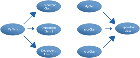
There are different levels of coupling, but let’s look at two types: afferent coupling and efferent coupling. Like the words used to describe them, there isn’t much difference between them. From the perspective of a given class, afferent coupling asks this question: how many classes depend on me? Efferent coupling asks the reverse question: upon how many classes do I depend? Figure 5.2 shows the difference.
Figure 5.2. Efferent coupling (left) tells you how many classes your class depends on. Afferent coupling (right) shows how many classes depend on your class.
Usually, you want your classes to be loosely coupled. For example, your classes shouldn’t depend on concrete implementations of other classes. You should shoot for a low value for your coupling statistics.
Higher coupling usually indicates a codebase that will be resistant to change. It’s not that you won’t be able to change that codebase, but the change you try to make will usually require significant ancillary changes. This outcome is also known as the ripple effect. It’s this ripple effect through the code that you want to minimize for the sake of maintainability. You’ve worked on a change to a system where you believe the impact will be minimal, but once we’re set into it, the tentacles of change start to reach further and further. We’ve all been there. The ripple effect is one of those code problems that can cause significant maintenance nightmares and, ultimately, high costs. Unfortunately, this effect happens far too often in brownfield projects.
In part 2, and especially chapter 9, we’ll discuss specific methods of reducing class coupling. Hint: Your classes should rely on interfaces more than they should concrete classes.
Once you’ve determined the likeliness of these ripples occurring when changes are attempted in your code, you need to know why that is. One of the reasons can be a lack of cohesion in the classes.
5.2.4. Cohesion
Somewhat related to coupling is cohesion. If a class is highly cohesive, its functions and responsibilities are closely related. If the class’s responsibilities are more disparate, it’s said to have low cohesion.
Experience has shown that an application that has a large number of low-cohesion classes often is harder to maintain than one with more cohesion. Low cohesion leads to cases where seemingly small changes must touch a lot of classes, leading to a more fragile environment. In addition, classes that aren’t cohesive tend to be harder to understand, and you end up spending a lot of time navigating through various classes trying to find the code that’s relevant to the task you’re working on.
Despite efforts to quantify it, cohesion is more subjective than other metrics. The reason is that closely related can mean different things to different people. For example, is it more cohesive to group functions by horizontal layers (data access, business logic, UI) or by vertical slice (all functions related to adding a customer, all functions related to searching for orders, etc.)?
Also, how finely grained do you make your classes? A single class called DataAccess isn’t going to win any cohesion awards, but on the other end of the spectrum, should you have a class for each possible database call?
Despite this ambiguity, there have been attempts to measure cohesion, or at least guide you toward better cohesion. Figure 5.3 shows a dependency matrix from the software tool NDepend (described later) which can be a useful indicator. There are also a few academic formulas designed to help assess cohesion, but in our experience, cohesion tends to increase naturally as you tackle other, more measurable metrics and introduce better coding practices in general.
Figure 5.3. A dependency matrix (shown here from NDepend[1]) can help assess cohesion. Squares around the diagonal suggest higher cohesion.

Examples of classes with low cohesion are the ubiquitous classes called Utility, StringFunctions, Global, or something similar. These classes typically contain numerous useful little utility functions that can be used application-wide. With the release of extension methods in .NET 3.5, these classes have become that much more prevalent.
Web services are often weakly cohesive as well. Often, methods are grouped together into a single web service for the sake of convenience to reduce the overhead of having to create references to multiple services.
The argument for high cohesion isn’t to say that you should throw away your HelperMethods classes or break out your web services into individual classes. Like with most other metrics, it’s impractical to eliminate low cohesion entirely. You can only learn to recognize when it’s causing a problem in your application.
As has been mentioned before, there isn’t one metric that provides all the answers. With cohesion, there’s a possibility that some of the measures can be somewhat more subjectively applied. As you’ll see in the discussion of the next metric, even the terms themselves become more subjective.
5.2.5. Distance from main sequence
Part of the appeal of the distance from main sequence metric is that you get to use terms like zone of pain and zone of uselessness in conversation. In fact, it’s a combination of two other metrics: abstractness and instability.
Abstractness and instability should be intuitive. Abstractness (abbreviated A) measures how many of your internal types are abstract (or interfaces) compared with the total number of types. It ranges between an assembly with no abstract classes or interfaces (A = 0) and one where there are no concrete classes (A = 1).
Instability is a comparison of efferent coupling (the number of types on which the assembly depends) to the total coupling. The following formula demonstrates this concept in mathematical terms (Ce stands for efferent coupling, and Ca stands for afferent coupling):
![]()
In less theoretical terms, instability is just a measure of how stable the assembly is, as you’d expect from the name.
From the formula, you can see that a high efferent coupling will increase an assembly’s instability. Intuitively, if your assembly depends on a lot of other assemblies, it means you may have to alter it if any of those dependent assemblies change. Conversely, a high afferent coupling means a lot of assemblies depend on this one, so you’re less likely to change it and break those dependencies. Your assembly is more stable in the sense that if it’s refactored, a lot of code will be affected. Instability is also measured on a range of 0 (stable) to 1 (instable).
A theoretically ideal assembly will have its abstractness and instability total to 1. The assembly is said to have a good balance between abstractness and instability in this case. When A + I = 1, this is known as the main sequence.
With this background behind us, the distance from the main sequence (abbreviated D) is just what it sounds like: how far is your assembly from this idealized main sequence?
This concept is easiest to see with a graph, shown in figure 5.4.
Figure 5.4. A graph of the distance from the main sequence taken from NDepend. Notice the Common assembly nestled in the Zone of Pain indicating that it contains a high number of concrete assemblies and that many assemblies depend on it.
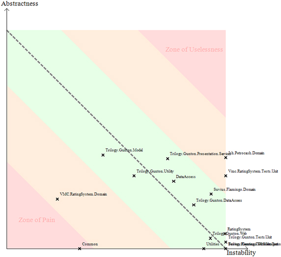
Notice the two labeled areas. The Zone of Uselessness indicates that your assembly is abstract and instable. This means there are a lot of abstract classes or interfaces that are highly dependent on external types, which is, as you would expect, pretty useless.
At the other end of the spectrum, you have classes that are concrete and have a lot of other assemblies relying on them. There are many types that depend on your classes, but your classes are concrete and, therefore, not very extensible. Hence, the Zone of Pain.
None of us wants the legacy of their code to be useless or painful to work with. Although the exact formula and the exact ratio number is calculable for this metric, we suggest that it be used as a delta metric. We don’t care so much about the exact value of the metric, but how it changes over time along with code changes. If during one month of development effort you see that a specific module has moved closer to the zone of pain, it should be an indication that a problem may be lurking.
Continuing with our trend to quantifiable, but subjective metrics, let’s take a look at an identifier that the development community is perhaps far too enamored with. The shocker is that it’s based on one of the pillars of object-oriented programming.
5.2.6. Depth of inheritance
This metric shows how many levels, or how deep, a particular class goes in its inheritance hierarchy. It’s a measure of how many base classes a particular class has. This metric is often referred to as a depth of inheritance tree (DIT).
Classes with a high depth of inheritance are generally more complex and harder to maintain than those with a lower depth. The reason is that as you increase the depth, you add more and more methods and properties to the class. But by the same token, it also means inherited methods will likely be reused more often by derived classes.
Use caution when basing decisions on this metric. More than the other metrics that have been mentioned, this metric isn’t meant for hard rules such as “No class will have a DIT higher than 5,” for example. Inheriting from System.Web.UI.UserControl, for instance, automatically means you have a DIT of 4.
Instead, this metric should be used to flag potential trouble spots. If a class has a DIT of 7, it should certainly be examined closely for a possible refactoring. But if upon close inspection you can justify the hierarchy, and if a better solution isn’t available, you should feel no guilt in leaving it as is.
Now that you’ve learned about a number of individual metrics, let’s take a look at how they can be used in combination.
5.2.7. Maintainability Index
This metric has an intuitive and seductive name—intuitive in that it’s a measure of how maintainable the code is—and seductive in that there’s some quantifiable way to measure what’s inherently a qualitative metric.
The formula for the Maintainability Index looks like this:
MI = 171 – (5.2 × 1n(HV)) – (0.23 × CycCom) – (16.2 × 1n(LOC))
In this equation, HV is the Halstead Volume (a measure of the code’s complexity weighted toward computational complexity), CycCom is the cyclomatic complexity of the code, and LOC is the number of lines of code. An optional component has been omitted that’s based on the number of comments in the code.
Lines of code antipattern
One metric that’s often brought up is the number of lines of code in an assembly, a class, or the application as a whole.
This metric is an easy one to comprehend. You simply count the number of lines of code (LOC). Of course, it’s easy to inflate your physical LOC count artificially so typically, when talking about LOC, reference is being made to logical lines—the number of lines of code as the compiler sees it.
We’re calling it out here because it’s rarely of any use within a brownfield project. It’s mostly a throwback to the 1980s when programmers were paid by the LOC. These days, the number of lines of code one has written is typically used only in a sort of perverse version of “pissing for distance” when egos are running hot. These days, it has some value as a means of comparing similar projects, but for our purposes, LOC isn’t a metric that produces anything actionable.
The simple fact is that there are many ways to code almost every piece of code. If one method of solving a problem has more LOC than another, it doesn’t explicitly mean that the code with the large LOC count is better. Many other factors, such as readability, maintainability, and correctness, play a much more important role than the number of LOC.
In today’s world of productivity utilities, code-generation tools, and autoformatting templates, LOC isn’t an informative indicator of anything other than possibly how much typing you’ve done. It’s mentioned because it’s often brought up by people bent on assigning more value to it than is necessary.
The complicated and seemingly random nature of this formula should raise some concerns as to its usefulness, especially when determining something as subjective as how maintainable an application is. Indeed, the data that was used to determine this formula predates .NET by a half decade or more.
If the statistical package you’re using includes this metric (like Visual Studio Code Metrics), it may be of academic interest. Its day-to-day usefulness is limited, which brings us to our next topic: becoming a slave to the statistics.
5.3. Becoming a slave to statistics
It’s easy to get wrapped up in code metrics. For example, there are many opinions on what constitutes sufficient code coverage. Some say you should strive for 100 percent code coverage. Others say that’s not only an inefficient goal, but it’s an impossible one in most cases. They would suggest that coverage of 75 percent may be more adequate and appropriate for your needs.
Regardless, once you wire code metrics into your build process, you may be surprised at the effect it has on you and some of your team members. Once you have a baseline level of statistics, developers may become draconian in maintaining it.
The extreme version of this is when the development team is so concerned with the statistics that they act with them specifically in mind, regardless of whether it’s for the good of the project.
For example, assume you’ve implemented your automated build so that it fails when your code coverage goes below a certain level, say 80 percent. Let’s also say your code currently sits at 81 percent coverage.
One day, during a massive refactoring, you discover that there’s a whole section of code that’s no longer needed. The problem is that this code is 100 percent covered by unit tests. And the codebase is small enough so that when you remove this code, the overall code coverage will drop to 79 percent, thus failing the build.
You can handle this situation in one of three ways:
- Roll back your changes so that the useless code remains but the code coverage remains above 80 percent.
- Retrofit some tests on existing code until the code coverage returns to 80 percent.
- Lower the code coverage limit.
If you choose either of the first two options, you may be taking your love of statistics too far. The reason for having a code coverage limit in place is to discourage any new code being checked in without corresponding tests. Remember from chapter 4 that our recommendation was to write tests on new or changed code only. But in this situation, that hasn’t happened. From an overall maintainability standpoint, you’re doing a good thing by removing unnecessary code. The fact that code coverage has gone down is a valid consequence of this.
The correct thing to do is to choose the third option: lower the code coverage limit so that the build doesn’t fail. This way, you can still check in your changes but you don’t need to focus on a superfluous task, like adding unit tests specifically to maintain code coverage. Yes, you’ve lowered your code coverage limit, but you’ve maintained the underlying intent of the metric.
This example underscores a larger point: avoid having your automated build process be dependent on any particular statistic, whether it’s code coverage, class coupling, or some other statistic. Unless you’re using a metric to enforce an aspect of your architecture, you shouldn’t have the build fail when a statistic drops to a certain level.
One reason for this has already been mentioned: there may be valid reasons for a drop in the metric. But more fundamentally, the practice keeps developers too focused on code metrics when they should be concentrating on the code.
Tales from the trenches: Tracer bullets
When first joining a large brownfield project, we had a number of options to choose from to get ourselves comfortable with the codebase and the issues we may have inherited with it. One of the techniques we could’ve used was to wade through the code in the development environment, but we would’ve missed large portions of both the codebase and the architecture. Instead, we took our first look at the code through the eyes of metrics.
After running a code metrics tool (in this case, NDepend) against the codebase, we had a much better idea of the areas we should look into further. These were portions of the application that were flagged as being highly coupled and possibly having excess complexity. Once we’d seen the general groupings of issues, we had a rough idea of where in the application possible problems could crop up. Note that we said could. In effect, what we’d done by gathering metrics on the codebase was to start firing tracer bullets.
For those unfamiliar with the term, tracer bullets are ammunition rounds that have been modified to include a pyrotechnic component that lights when the round is fired, making it easy to see in flight. By reviewing the trajectory of the round, shooters can adjust their aim to be more accurate.
Using code metrics as tracer bullets allows us to get a rough idea of where issues exist in the codebase. We can use the information we gather as a tool to help direct our changes so that development effort can be properly focused to achieve the project’s end goals (quality, maintainability, replaceability, reversibility). The primary goal of tracer rounds, and metrics, isn’t to inflict direct hits. Instead, we use them to refine our efforts.
In our project, we combined the metrics we gathered with current and past information from our defect-tracking system (see chapter 6) to refine our knowledge of the issues that the project was facing. Based on that combined information, we were able to refine the development efforts. The tracers we fired pointed us toward a quality and stability issue in the system.
Once we’d performed this ritual a couple of times in the project, we slightly shifted the focus of what we were gleaning from the metric reports. Instead of looking for specific numbers on certain metrics, we shifted to reviewing the delta in each metric that we felt was important to achieving our goals. For example, we felt that coupling was causing significant code stability issues on the project. Instead of saying that we wanted to achieve an efferent coupling value of, say, 2 in a certain module, we looked at the change from one salvo of tracer bullets to the next. Because we were actively working to improve coupling, we expected to see it lowering with each iteration. If we noted that the value didn’t change or had increased, we immediately flagged the metric for investigation.
For us, using metrics as a guide and a delta measurement proved to be an effective way to gain a strong understanding of the direction that our coding efforts needed to take. By themselves, the metrics didn’t indicate this. The true value came from combining metrics, their deltas over time, defect entry–based information, and the knowledge of the end goal we were trying to achieve.
In short, software metrics are there for guidance, not process. It’s useful to monitor them at regular intervals and make decisions and adjustments based on them, but they shouldn’t be part of your day-to-day activities. We’ll expand on this idea later in this chapter after you’ve learned how to provide easy access to the analysis metrics through integration with our build process.
5.4. Implementing statistical analysis
Now that you’ve been warned not to focus on statistics, the natural progression is to outline how to automate their generation.
Here comes the bad news: unlike most of the tools covered so far, the most common tools used to perform statistical analysis on your code aren’t free. But for the optimists in the crowd who need a silver lining, with a commercial product comes technical support, should you need it. And there still exists the stigma in many organizations that if the tool is free, it has no place on the company servers.
For code coverage, the de facto standard for .NET applications is NCover, which only recently became a commercial product. The older, free version is still readily available, though it predates .NET 3.5 and doesn’t work completely with the new features. Visual Studio Team System also includes a code coverage utility, but it isn’t as easily integrated into an automated build as NCover is.
For the rest of the code metrics, you could use the Code Metrics feature in either Visual Studio Team Developer or Team Suite. At present, both calculate five metrics: Maintainability Index, Cyclomatic Complexity, Depth of Inheritance, Class Coupling, and Lines of Code. At the time of this writing, Code Metrics is available only for Visual Studio 2008.
Alternatively, NDepend will provide the same statistics plus several dozen more,[1] and it’s available for earlier versions of Visual Studio. NDepend also provides more reporting capabilities to help you zero in on trouble spots in your code. Like NCover, NDepend is a commercial product requiring purchased licenses.
Both NDepend and NCover are easily incorporated into an automated build and your CI process. Both come with tasks that can be used with NAnt or MSBuild, and there are plenty of examples of how to weave the output from each of them into popular CI products, like the open source CruiseControl.NET or JetBrains’ TeamCity.
5.4.1. Automating code coverage
As mentioned earlier, code coverage is useful primarily as a mechanism for evaluating how well your code is covered by tests. The implicit dependency here is that both your application and the test project(s) should be compiled. Therefore, the process that needs automation consists of these steps:
1.
Compile the application.
2.
Compile the tests.
3.
Execute the code coverage application against the unit-testing utility, passing in the test assembly as an argument.
If you’ve made it this far in the book, steps 1 and 2 should already be done in your automated build, leaving only automation of the code coverage application. Any code coverage utility worth its salt will have a command-line interface, so automation is simply a matter of executing it with the appropriate parameters.
Notice that two applications are being executed in step 3. Code coverage utilities usually involve connecting to a running application so they can monitor the methods being covered. Recall from chapter 4, you connect up to the unit-testing application to execute our unit and integration tests while the code coverage utility watches and logs.
Listing 5.2 shows a sample NAnt target that will execute NCover on a test assembly.
Listing 5.2. Sample NAnt target executing NCover for code coverage
<target name="coverage" depends="compile test.compile">
<exec program="${path.to.ncover.console.exe}">
<arg value="//w "${path.to.build.folder}"" />
<arg value="//x "${path.to.output.file}" />
<arg value=""${path.to.nunit.console}"" />
<arg value="${name.of.test.assembly}
/xml:${path.to.test.results.file}" />
</exec>
</target>
Notice that a dependency has been added on the compile and test.compile targets to ensure that the application code and the test project are compiled before executing NCover.
Code coverage: Two processes for the price of one?
As you can see from the sample target in listing 5.2, you end up with two output files: one with the test results and one with the code coverage results. This is because you actually are executing your tests during this task.
You don’t technically need to execute your tests in a separate task if you’re running the code coverage task. For this reason, many teams will substitute an automated code coverage task for their testing task, essentially performing both actions in the CI process. The CI server will compile the code, test it, and generate code coverage stats on every check-in.
Although there’s nothing conceptually wrong with this approach, be aware of some downsides. First, there’s overhead to generating code coverage statistics. When there are a lot of tests, this overhead could be significant enough to cause friction in the form of a longer-running automated build script. Remember that the main build script should run as fast as possible to encourage team members to run it often. If it takes too long to run, you may find developers looking for workarounds.
For these reasons, we recommend executing the code coverage task separately from the build script’s default task. It should be run at regular intervals, perhaps as a separate scheduled task in your build file that executes biweekly or even monthly, but we don’t feel there’s enough benefit to the metric to warrant the extra overhead of having it execute on every check-in.
Also note that NCover is being connected to the NUnit console application. That way, when this task is executed NCover will launch the NUnit console application, which will execute all the tests in the specified assembly. The test results will be stored in the file specified by the ${path.to.test.results.file} variable (which is set elsewhere in the build file).
Now let’s see how we can automate other metrics.
5.4.2. Automating other metrics
Automating the generation of code metrics is similar to generating code coverage statistics: you execute an application. The only difference is the application you execute and the arguments you pass.
The following snippet is an NAnt task that will execute code analysis using NDepend:
<target name="code-metrics" depends="compile">
    <exec program="${path.to.ndepend.console.exe}">
      <arg value="${path.to.ndepend.project.xml.file}" />
    </exec>
</target>
Unlike the code coverage task, this one depends only on the compile target, which means the application must be compiled before the task can be executed. Doing so ensures that the metrics run against the current version of the code on the machine. Also note that NDepend includes a custom <ndepend> NAnt task that can be used as an alternative to <exec>.
Why separate code coverage?
Some of you may be asking why we’re singling out code coverage for special attention.
Conceptually, there’s no reason why code coverage should be treated any differently than other metrics. One could make an argument that it’s a more useful metric (or at least an easier one to understand), but it’s just another statistic.
The reason is tool availability. At the time of this writing, NCover is the standard for code coverage for all intents and purposes. Until recently, it was a free tool, which helped make it somewhat ubiquitous. That, and the intuitive nature of code coverage, has pushed code coverage to a level of heightened awareness.
By contrast, utilities that generate other metrics, such as NDepend, aren’t as prevalent. Whether it’s due to the fact that these tools have a cost associated or whether the underlying statistics aren’t as readily actionable as code coverage, the fact remains that tools are commonly used for code coverage, but not so much for other metrics.
This task may seem on the sparse side considering the work to be performed. For example, there isn’t even an argument for the output file. The reason is the implementation details are hidden in the argument, the NDepend project file. This file contains details of the metrics you’d like measured, the output XML file, and any Code Query Language (CQL) statements to be executed. CQL is an NDepend-specific querying language that allows you to raise warnings if metrics don’t meet a certain standard. For example, you could fail the build if, say, your afferent coupling was higher than 20.
A full description of the NDepend project file is outside of the scope of this book. Our goal is to show how you could automate such a tool in your build file. As you can see, it’s as simple as executing an application.
But before you start integrating code metrics into your CI process, we have some opinions on the topic that you should hear.
5.4.3. Metrics with CI
Now that you’ve briefly read about incorporating code coverage into your CI process and we’ve touched on our opinion about this topic, let’s expand on that concept with this question: how do you integrate code metrics into your CI process?
The answer is, you don’t.
You don’t generate code metrics on every check-in the same way you compile and test your code. Generating statistics can be time consuming, and the incremental value of doing it on every check-in is minimal. And as mentioned in section 5.3, you risk encouraging bad habits in yourself and your development team.
Instead, consider having a separate (but still automated) process specifically for analyzing your codebase. It could be scheduled to run once a week or twice a month or some other interval or only through manual triggering, but make sure it’s a large enough one that you can see meaningful changes from one run to the next.
The task will be closely related to your CI process. For example, the NAnt targets you use to generate statistics will likely sit alongside the targets that compile and test the applications. But they won’t execute as part of the regular check-in process. Rather, you can create a separate task that executes these targets on a schedule rather than on a check-in trigger.
When you do this, you can start monitoring trends in your application. For example, if your code coverage increases at a steady pace, then starts slowing (or even dropping), that’s a sign of something that needs attention.
We’ll provide a more in-depth discussion on trending in the next chapter when we’re looking at defects.
In the beginning, you may want to monitor the metrics more often, if only for the psychological effect you’ll achieve in seeing the numbers improve early in the project. As the code progresses, the improvements will become more marginal and you’ll get into a rhythm that increases your stats naturally. It’s still a good idea to monitor them on occasion, just to make sure you’re still on track. But at that point, you’re looking more for discrepancies. Checking your metrics should be a matter of comparing them to the trend to see if they’re in line. If so, move on. If not, do your investigative work to see if corrective action is necessary.
Before closing, and since there’s space available, this is a good spot for a quick discussion of other tasks that could be automated in your build process.
5.5. Other tasks for automation
Code metrics aren’t the only things that can be automated. As you can probably tell from our NCover and NDepend examples, you can automate any application, provided it can run unattended.
Just as with code metrics and tests, you’ll need to decide not only whether the task is important enough to automate, but also whether it should be incorporated into your CI process. Start with the assumption that any task other than automated unit tests should be excluded from your CI process unless you’re feeling friction because of its omission.
Here’s a list of processes that could be automated (along with suggested applications for performing the operation):
- Generating documentation from XML comments (Sandcastle or Docu)
- Enforcing coding standards (FxCop or StyleCop)
- Check for duplication in your code (Simian – Similarity Analyser)
- Code generation (CodeSmith or MyGeneration)
- Data migrations, test database creation (SQL Data Compare/SQL Packager, SQL scripts)
You should be on the lookout for tasks that can be automated, even if it’s simply executing a batch file to copy files from one place to another. The benefits of reducing the possibility of errors and keeping yourself focused on useful tasks should be readily apparent.
Like with CI in chapter 3, our goal with this brief section was twofold: to give you some ideas as to what to automate but also to kick-start your thought process. Is there anything you have to do manually and by rote to build your application? In many brownfield applications, the answer is yes. Often regular tasks creep into the build process without us realizing it. At one point, maybe you decided to generate documentation from the code. Then you did it again, then again and again until it became part of the regular process. Surely someone thought “Why am I doing this?” but has anyone thought, “Why aren’t we automating this?”
5.6. Summary
The honeymoon is over. We spent the better part of chapter 1 convincing you that working on a brownfield application is an exciting endeavor. Working through the next chapters, you’ve made some tremendous headway by installing a CI process, automating your tests, and setting a foundation for future development.
But now you’ve been hit with a dose of reality. In this chapter, you took your first hard look at the state the application is in. You examined some code metrics, such as code coverage, class coupling, and cyclomatic complexity, and learned how to automate them.
When you take your first look at the statistics for the software metrics you’ve entered, the initial numbers might be overwhelming. And let’s face it: there’s no encouraging way to say “We’re neck deep in the zone of pain.”
Like the tortoise, slow and steady wins the race. You read about using the reports to zero in on problem areas and to identify refactoring points that will give you the most bang for your buck. Once they’ve been singled out, all that’s left is how to deal with them. That’s where part 2 comes in.
In part 2, we’ll talk extensively on various techniques that will make the software more maintainable. Coupled with the tests you’re writing for all new code, you’ll find that the numbers become more palatable on their own without requiring a directed effort to, say, reduce coupling.
There’s one final chapter before we dive into some code. This one involves managing the defects and feature requests that come in from your testing department and users. Between the code metrics and the defect/feature requests, you’ll be able to make informed decisions on how to convert this brownfield application into something manageable.