
Cluster analysis is the process of grouping objects together in a way that objects in one group are more similar than objects in other groups.
An example would be identifying and grouping clients with similar booking activities on a travel portal, as shown in the following figure.
In the preceding example, each group is called a cluster, and each member (data point) of the cluster behaves in a manner similar to its group members.
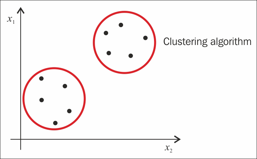
Cluster analysis
Cluster analysis is an unsupervised learning method. In supervised methods, such as regression analysis, we have input variables and response variables. We fit a statistical model to the input variables to predict the response variable. Whereas in unsupervised learning methods, however, we do not have any response variable to predict; we only have input variables. Instead of fitting a model to the input variables to predict the response variable, we just try to find patterns within the dataset. There are three popular clustering algorithms: hierarchical cluster analysis, k-means cluster analysis, and two-step cluster analysis. In the following section, we will learn about k-means clustering.
k-means is an unsupervised, iterative algorithm where k is the number of clusters to be formed from the data. Clustering is achieved in two steps:
- Cluster assignment step: In this step, we randomly choose two cluster points (red dot and green dot) and assign each data point to the cluster point that is closer to it (top part of the following image).
- Move centroid step: In this step, we take the average of the points of all the examples in each group and move the centroid to the new position, that is, mean position calculated (bottom part of the following image).
The preceding steps are repeated until all the data points are grouped into two groups and the mean of the data points after moving the centroid doesn't change.
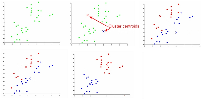
Steps of cluster analysis
The preceding image shows how a clustering algorithm works on data to form clusters. See the R implementation of k-means clustering on iris dataset as follows:
#k-means clustering
library(cluster)
data(iris)
iris$Species = as.numeric(iris$Species)
kmeans<- kmeans(x=iris, centers=5)
clusplot(iris,kmeans$cluster, color=TRUE, shade=TRUE,labels=13, lines=0)
The output of the preceding code is as follows:
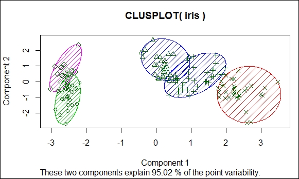
Cluster analysis results
The preceding image shows the formation of clusters on the iris data, and the clusters account for 95 percent of the data. In the preceding example, the number of clusters of k value is selected using the elbow method, as shown here:
library(cluster)
library(ggplot2)
data(iris)
iris$Species = as.numeric(iris$Species)
cost_df <- data.frame()
for(i in 1:100){
kmeans<- kmeans(x=iris, centers=i, iter.max=50)
cost_df<- rbind(cost_df, cbind(i, kmeans$tot.withinss))
}
names(cost_df) <- c("cluster", "cost")
#Elbow method to identify the idle number of Cluster
#Cost plot
ggplot(data=cost_df, aes(x=cluster, y=cost, group=1)) +
theme_bw(base_family="Garamond") +
geom_line(colour = "darkgreen") +
theme(text = element_text(size=20)) +
ggtitle("Reduction In Cost For Values of 'k'
") +
xlab("
Clusters") +
ylab("Within-Cluster Sum of Squares
")
The following image shows the cost reduction for k values:
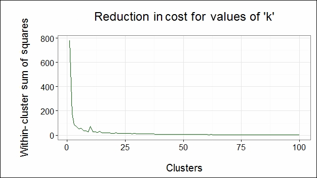
From the preceding figure, we can observe that the direction of the cost function is changed at cluster number 5. Hence, we choose 5 as our number of clusters k. Since the number of optimal clusters is found at the elbow of the graph, we call it the elbow method.
Support vector machine algorithms are a form of supervised learning algorithms employed to solve classification problems. SVM is generally treated as one of the best algorithms to deal with classification problems. Given a set of training examples, where each data point falls into one of two categories, an SVM training algorithm builds a model that assigns new data points into one category or the other. This model is a representation of the examples as a points in space, mapped so that the examples of the separate categories are divided by a margin that is as wide as possible, as shown in the following image. New examples are then mapped into that same space and predicted to belong to a category based on which side of the gap they fall on. In this section, we will go through an overview and implementation of SVMs without going into mathematical details.
When SVM is applied to a p-dimensional dataset, the data is mapped to a p-1 dimensional hyperplane, and the algorithm finds a clear boundary with a sufficient margin between classes. Unlike other classification algorithms that also create a separating boundary to classify data points, SVM tries to choose a boundary that has the maximum margin to separate the classes, as shown in the following image:
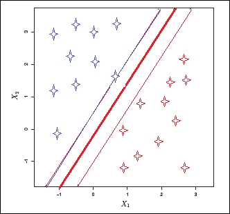
Consider a two-dimensional dataset having two classes, as shown in the preceding image. Now, when the SVM algorithm is applied, first it checks whether a one-dimensional hyperplane exists to map all the data points. If the hyperplane exists, the linear classifier creates a decision boundary with a margin to separate the classes. In the preceding image, the thick red line is the decision boundary, and the thinner blue and red lines are the margins of each class from the boundary. When new test data is used to predict the class, the new data falls into one of the two classes.
Here are some key points to be noted:
- Though an infinite number of hyperplanes can be created, SVM chooses only one hyperplane that has the maximum margin, that is, the separating hyperplane that is farthest from the training observations.
- This classifier is only dependent on the data points that lie on the margins of the hyperplane, that is, on thin margins in the image, but not on other observations in the dataset. These points are called support vectors.
- The decision boundary is affected only by the support vectors but not by other observations located away from the boundaries. If we change the data points other than the support vectors, there would not be any effect on the decision boundary. However, if the support vectors are changed, the decision boundary changes.
- A large margin on the training data will also have a large margin on the test data to classify the test data correctly.
- Support vector machines also perform well with non-linear datasets. In this case, we use radial kernel functions.
See the R implementation of SVM on the iris dataset in the following code snippet. We used the e1071 package to run SVM. In R, the SVM() function contains the implementation of support vector machines present in the e1071 package.
Now, we will see that the SVM() method is called with the tune() method, which does cross validation and runs the model on different values of the cost parameters.
The cross-validation method is used to evaluate the accuracy of the predictive model before testing on future unseen data:
  #SVM
library(e1071)
data(iris)
sample = iris[sample(nrow(iris)),]
train = sample[1:105,]
test = sample[106:150,]
tune =tune(svm,Species~.,data=train,kernel ="radial",scale=FALSE,ranges =list(cost=c(0.001,0.01,0.1,1,5,10,100)))
tune$best.model
Call:
best.tune(method = svm, train.x = Species ~ ., data = train, ranges = list(cost = c(0.001,
0.01, 0.1, 1, 5, 10, 100)), kernel = "radial", scale = FALSE)Parameters:
   SVM-Type:  C-classification
 SVM-Kernel:  radial
       cost:  10
      gamma:  0.25

Number of Support Vectors:  25

summary(tune)

Parameter tuning of 'svm':
- sampling method: 10-fold cross validation
- best parameters:
 cost
   10
- best performance: 0.02909091
- Detailed performance results:
   cost      error dispersion
1 1e-03 0.72909091 0.20358585
2 1e-02 0.72909091 0.20358585
3 1e-01 0.04636364 0.08891242
4 1e+00 0.04818182 0.06653568
5 5e+00 0.03818182 0.06538717
6 1e+01 0.02909091 0.04690612
7 1e+02 0.07636364 0.08679584

model =svm(Species~.,data=train,kernel ="radial",cost=10,scale=FALSE)
// cost =10 is chosen from summary result of tune variable
The tune$best.model object tells us that the model works best with the cost parameter as 10 and total number of support vectors as 25:
pred = predict(model,test)