
Decision trees are a simple, fast, tree-based supervised learning algorithm to solve classification problems. Though not very accurate when compared to other logistic regression methods, this algorithm comes in handy while dealing with recommender systems.
We define the decision trees with an example. Imagine a situation where you have to predict the class of flower based on its features such as petal length, petal width, sepal length, and sepal width. We will apply the decision tree methodology to solve this problem:
- Consider the entire data at the start of the algorithm.
- Now, choose a suitable question/variable to divide the data into two parts. In our case, we chose to divide the data based on petal length > 2.45 and <= 2.45. This separates flower class
setosafrom the rest of the classes. - Now, further divide the data having petal length >2.45, based on the same variable with petal length < 4.5 and >= 4.5, as shown in the following image.
- This splitting of the data will be further divided by narrowing down the data space until we reach a point where all the bottom points represent the response variables or where further logical split cannot be done on the data.
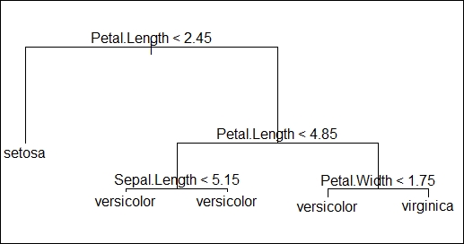
In the following decision tree image, we have one root node, four internal nodes where data split occurred, and five terminal nodes where data split cannot be done any further. They are defined as follows:
- Petal.Length <2.45 as root node
- Petal.Length <4.85, Sepal.Length <5.15, and Petal.Width <1.75 are called internal nodes
- Final nodes having the class of the flowers are called terminal nodes
- The lines connecting the nodes are called the branches of the tree
While predicting responses on new data using the previously built model, each new data point is taken through each node, a question is asked, and a logical path is taken to reach its logical class, as shown in the following figure:
See the decision tree implementation in R on the iris dataset using the tree package available from Comprehensive R Archive Network (CRAN).
The summary of the mode is given here. It tells us that the misclassification rate is 0.0381, indicating that the model is accurate:
library(tree)
data(iris)
sample = iris[sample(nrow(iris)),]
train = sample[1:105,]
test = sample[106:150,]
model = tree(Species~.,train)
summary(model)
Classification tree:
tree(formula = Species ~ ., data = train, x = TRUE, y = TRUE)
Variables actually used in tree construction:
[1] "Petal.Length" "Sepal.Length" "Petal.Width"
Number of terminal nodes:  5
Residual mean deviance:  0.1332 = 13.32 / 100
Misclassification error rate: 0.0381 = 4 / 105 '
//plotting the decision tree
plot(model)text(model)
pred = predict(model,test[,-5],type="class")
> pred
 [1] setosa     setosa     virginica  setosa     setosa     setosa     versicolor
 [8] virginica  virginica  setosa     versicolor versicolor virginica  versicolor
[15] virginica  virginica  setosa     virginica  virginica  versicolor virginica
[22] versicolor setosa     virginica  setosa     versicolor virginica  setosa
[29] versicolor versicolor versicolor virginica  setosa     virginica  virginica
[36] versicolor setosa     versicolor setosa     versicolor versicolor setosa
[43] versicolor setosa     setosa
Levels: setosa versicolor virginica