We will build the model using a part of the MovieLense dataset (the training set) and apply it on the other part (the test set). Since it's not a topic of this chapter, we will not evaluate the model, but will only recommend movies to the users in the test set.

The two sets are as follows:

The algorithm automatically normalizes the data, so we can use ratings_movies that contains relevant users and movies of MovieLense. We defined ratings_movies in the previous section as the subset of MovieLense users who have rated at least 50 movies and movies that have been rated at least 100 times.

First, we randomly define the which_train vector that is TRUE for users in the training set and FALSE for the others. We will set the probability in the training set as 80 percent:

which_train <- sample(x = c(TRUE, FALSE), size = nrow(ratings_movies), replace = TRUE, prob = c(0.8, 0.2))
head(which_train)
## [1]  TRUE  TRUE  TRUE FALSE  TRUE FALSE

Let's define the training and the test sets:

recc_data_train <- ratings_movies[which_train, ]
recc_data_test <- ratings_movies[!which_train, ]

If we want to recommend items to each user, we could just use the k-fold:

This is a sample code:

which_set <- sample(x = 1:5, size = nrow(ratings_movies), replace = TRUE)
for(i_model in 1:5) {
  which_train <- which_set == i_model
  recc_data_train <- ratings_movies[which_train, ]
  recc_data_test <- ratings_movies[!which_train, ]
  # build the recommender
}

In order to show how this package works, we split the data into training and test sets manually. You can also do this automatically in recommenderlab using the evaluationScheme function. This function also contains some tools to evaluate models that we will use in the Chapter 4, Evaluating the Recommender Systems, which is about model evaluation.

Now, we have the inputs to build and validate the model.

The function to build models is recommender and its inputs are as follows:

The model is called IBCF, which stands for item-based collaborative filtering. Let's take a look at its parameters:

recommender_models <- recommenderRegistry$get_entries(dataType = "realRatingMatrix")
recommender_models$IBCF_realRatingMatrix$parameters

Some relevant parameters are as follows:

At the moment, we can just set them to their defaults. In order to show how to change parameters, we are setting k = 30, which is the default. We are now ready to build a recommender model:

recc_model <- Recommender(data = recc_data_train, method = "IBCF", parameter = list(k = 30))recc_model
## Recommender of type 'IBCF' for 'realRatingMatrix' ## learned using 111 users.
class(recc_model)
## [1] "Recommender"
## attr(,"package")
## [1] "recommenderlab"

The recc_model class is an object of the Recommender class containing the model.

Using getModel, we can extract some details about the model, such as its description and parameters:

model_details <- getModel(recc_model)
model_details$description
## [1] "IBCF: Reduced similarity matrix"
model_details$k
## [1] 30

The model_details$sim component contains the similarity matrix. Let's check its structure:

class(model_details$sim)
## [1] "dgCMatrix"
## attr(,"package")
## [1] "Matrix"
dim(model_details$sim)
## [1] 332 332

As expected, model_details$sim is a square matrix whose size is equal to the number of items. We can explore a part of it using image:

n_items_top <- 20

Let's build the heat map:

image(model_details$sim[1:n_items_top, 1:n_items_top], main = "Heatmap of the first rows and columns")

The following image displays heatmap of the first rows and columns:

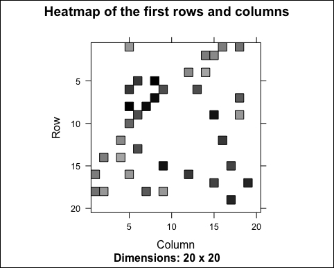
Most of the values are equal to 0. The reason is that each row contains only k elements. Let's check it:

model_details$k
## [1] 30
row_sums <- rowSums(model_details$sim > 0)
table(row_sums)
## row_sums
##  30
## 332

As expected, each row has 30 elements greater than 0. However, the matrix is not supposed to be symmetric. In fact, the number of non-null elements for each column depends on how many times the corresponding movie was included in the top k of another movie. Let's check the distribution of the number of elements by column:

col_sums <- colSums(model_details$sim > 0)

Let's build the distribution chart:

qplot(col_sums) + stat_bin(binwidth = 1) + ggtitle("Distribution of the column count")

The following image displays the distribution of the column count:

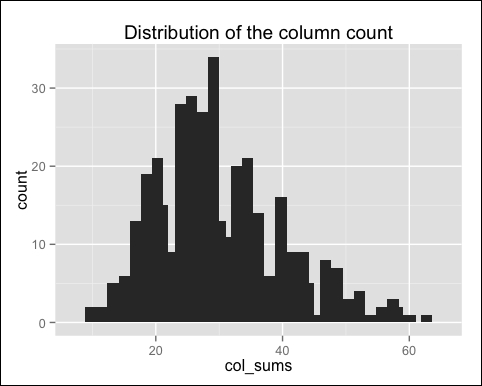
As expected, there are a few movies that are similar to many others. Let's see which are the movies with the most elements:

which_max <- order(col_sums, decreasing = TRUE)[1:6]
rownames(model_details$sim)[which_max]

Now, we are able to recommend movies to the users in the test set. We will define n_recommended that specifies the number of items to recommend to each user. This section will show you the most popular approach to computing a weighted sum:

n_recommended <- 6

For each user, the algorithm extracts its rated movies. For each movie, it identifies all its similar items, starting from the similarity matrix. Then, the algorithm ranks each similar item in this way:

Then, the algorithm identifies the top n recommendations:

recc_predicted <- predict(object = recc_model, newdata = recc_data_test, n = n_recommended)
recc_predicted
## Recommendations as 'topNList' with n = 6 for 449 users.

The recc_predicted object contains the recommendations. Let's take a look at its structure:

class(recc_predicted)
## [1] "topNList"## attr(,"package")## [1] "recommenderlab"
slotNames(recc_predicted)
## [1] "items"      "itemLabels" "n"

The slots are:

For instance, these are the recommendations for the first user:

recc_predicted@items[[1]]
## [1] 201 182 254 274 193 297

We can extract the recommended movies from recc_predicted@item labels:

recc_user_1 <- recc_predicted@items[[1]]movies_user_1 <- recc_predicted@itemLabels[recc_user_1]
movies_user_1

We can define a matrix with the recommendations for each user:

recc_matrix <- sapply(recc_predicted@items, function(x){
  colnames(ratings_movies)[x]
})
dim(recc_matrix)
## [1]   6 449

Let's visualize the recommendations for the first four users:

recc_matrix[, 1:4]

Now, we can identify the most recommended movies. For this purpose, we will define a vector with all the recommendations, and we will build a frequency plot:

number_of_items <- factor(table(recc_matrix))chart_title <- "Distribution of the number of items for IBCF"

Let's build the distribution chart:

qplot(number_of_items) + ggtitle(chart_title)

The following image shows the distribution of the number of items for IBCF:

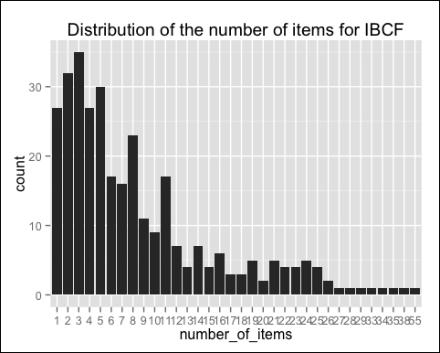
Most of the movies have been recommended only a few times, and a few movies have been recommended many times. Let's see which are the most popular movies:

number_of_items_sorted <- sort(number_of_items, decreasing = TRUE)
number_of_items_top <- head(number_of_items_sorted, n = 4)
table_top <- data.frame(names(number_of_items_top), number_of_items_top)
table_top

The preceding table continues as follows:

IBCF recommends items on the basis of the similarity matrix. It's an eager-learning model, that is, once it's built, it doesn't need to access the initial data. For each item, the model stores the k-most similar, so the amount of information is small once the model is built. This is an advantage in the presence of lots of data.

In addition, this algorithm is efficient and scalable, so it works well with big rating matrices. Its accuracy is rather good, compared with other recommendation models.

In the next section, we will explore another branch of techniques: user-based collaborative filtering.