
Classification and prediction are two important methods of data analysis used to find patterns in data. Classification predicts the categorical class (or discrete values), whereas regression and other models predict continuous valued functions. However, Logistic Regression addresses categorical class also. For example, a classification model may be built to predict the results of a credit-card application approval process (credit card approved or denied) or to determine the outcome of an insurance claim. Many classification algorithms have been developed by researchers and machine-learning experts. Most classification algorithms are memory intensive. Recent research has developed parallel and distributed processing architecture, such as Hadoop, which is capable of handling large amounts of data.
This chapter focuses on basic classification techniques. It explains some classification methods including naïve Bayes, decision trees, and other algorithms. It also provides examples using R packages available to perform the classification tasks.
6.1 What Is Classification? What Is Prediction?
Imagine that you are applying for a mortgage. You fill out a long application form with all your personal details, including income, age, qualification, location of the house, valuation of the house, and more. You are anxiously waiting for the bank’s decision on whether your loan application has been approved. The decision is either Yes or No. How does the bank decide? The bank reviews various parameters provided in your application form, and then— based on similar applications received previously and the experience the bank has had with those customers—the bank decides whether the loan should be approved or denied.
Now imagine that you have to make a decision about launching a new product in the market. You have to make a decision of Launch or No Launch. This depends on various parameters. Your decision will be based on similar experiences you had in the past launching products, based on numerous market parameters.
Next, imagine that you want to predict the opinions expressed by your customers on the products and services your business offers. Those opinions can be either positive or negative and can be predicted based on numerous parameters and past experiences of your customers with similar products and services.
Finally, imagine that airport authorities have to decide, based on a set of parameters, whether a particular flight of a particular airline at a particular gate is on time or delayed. This decision is based on previous flight details and many other parameters.
Classification is a two-step process. In the first step, a model is constructed by analyzing the database and the set of attributes that define the class variable. A classification problem is a supervised machine-learning problem. The training data is a sample from the database, and the class attribute is already known. In a classification problem, the class of Y, a categorical variable, is determined by a set of input variables {x1, x2, x3, …}. In classification, the variable we would like to predict is typically called class variable C, and it may have different values in the set {c1, c2, c3, …}. The observed or measured variables X1, X2, … Xn are the attributes, or input variables, also called explanatory variables. In classification, we want to determine the relationship between the Class variable and the inputs, or explanatory variables. Typically, models represent the classification rules or mathematical formulas. Once these rules are created by the learning model, this model can be used to predict the class of future data for which the class is unknown.
There are various types of classifier models: based on a decision boundary, based on probability theory, and based on discriminant analysis. We begin our discussion with a classifier based on the probabilistic approach. Then we will look at the decision trees and discriminant classifiers.
6.2 Probabilistic Models for Classification
Probabilistic classifiers and, in particular, the naïve Bayes classifier, is the most popular classifier used by the machine-learning community. The naïve Bayes classifier is a simple probabilistic classifier based on Bayes’ theorem, the most popular theorem in natural- language processing and visual processing. It is one of the most basic classification techniques, with applications such as e-mail spam detection, e-mail sorting, and sentiment analysis. Even though naïve Bayes is a simple technique, it provides good performance in many complex real-world problems.
The study of probabilistic classification is based on the study of approximating joint distribution with an assumption of independence and then decomposing this probability into a product of conditional probability. A conditional probability of event A, given event B—denoted by P(A|B)—represents the chances of event A occurring, given that event B also occurs.
In the context of classification, Bayes theorem provides a formula for calculating the probability of a given record belonging to a class for the given set of record attributes. Suppose you have m classes, C1, C2, C3, … Cm and you know the probability of classes P(C1), P(C2), … P(Cm). If you know the probability of occurrence of x1, x2, x3, … attributes within each class, then by using Bayes’ theorem, you can calculate the probability that the record belongs to class Ci:

P(Ci) is the prior probability of belonging to class Ci in the absence of any other attributes. (Ci|Xi) is the posterior probability of Xi belonging to class Ci. In order to classify a record using Bayes’ theorem, you compute its chance of belonging to each class Ci. You then classify based on the highest probability score calculated using the preceding formula.
It would be extremely computationally expensive to compute P(X|Ci) for data sets with many attributes. Hence, a naïve assumption is made that presumes that each record is independent of the others, given the class label of the sample. It is reasonable to assume that the predictor attributes are all mutually independent within each class, so we can simplify the equation:
![]()
Assume that each data sample is represented by an n-dimensional vector, X = {x1, x2, … xn}, samples from n attributes of categorical class values A1, A2, …. An with m classes C1, C2, … Cm, then P(Xk|Ci) = n/N, where n is the number of training samples of class Ci having value Xk for Ak, and N is the total number of training samples belonging to Ci.
6.2.1 Example
Let’s look at one example and see how to predict a class label by using a Bayesian classifier. Table 6-1 presents a training set of data tuples for a bank credit-card approval process .
Table 6-1. Sample Training Set
ID | Purchase Frequency | Credit Rating | Age | Class Label: Yes = Approved No = Denied |
|---|---|---|---|---|
1 | Medium | OK | < 35 | No |
2 | Medium | Excellent | < 35 | No |
3 | High | Fair | 35–40 | Yes |
4 | High | Fair | > 40 | Yes |
5 | Low | Excellent | > 40 | Yes |
6 | Low | OK | > 40 | No |
7 | Low | Excellent | 35–40 | Yes |
8 | Medium | Fair | < 35 | No |
9 | Low | Fair | < 35 | No |
10 | Medium | Excellent | > 40 | No |
11 | High | Fair | < 35 | Yes |
12 | Medium | Excellent | 35–40 | No |
13 | Medium | Fair | 35–40 | Yes |
14 | High | OK | < 35 | No |
The data samples in this training set have the attributes Age, Purchase Frequency, and Credit Rating. The class label attribute has two distinct classes: Approved or Denied. Let C1 correspond to the class Approved, and C2 correspond to class Denied. Using the naïve Bayes classifier, we want to classify an unknown label sample X:
X = (Age >40, Purchase Frequency = Medium, Credit Rating = Excellent)
To classify a record, first compute the chance of a record belonging to each of the classes by computing P(Ci|X1,X2, … Xp) from the training record. Then classify based on the class with the highest probability.
In this example, there are two classes. We need to compute P(Xi|Ci)P(Ci). P(Ci) is the prior probability of each class:
P(Application Approval = Yes) = 6/14 = 0.428
P(Application Approval = No) = 8/14 = 0.571
Let’s compute P(X|Ci), for i =1, 2, … conditional probabilities:
P(Age > 40 | Approval = Yes) = 2/6 = 0.333
P(Age > 40 | Approval = No) = 2/8 = 0.25
P(Purchase Frequency = Medium | Approval = Yes) =1/6 = 0.167
P(Purchase Frequency = Medium | Approval = No) = 5/8 = 0.625
P(Credit Rating = Excellent | Approval = Yes) = 2/6 = 0.333
P(Credit Rating = Excellent | Approval = No) = 3/8 = 0.375
Using these probabilities, you can obtain the following:
P(X | Approval = Yes) = 0.333 × 0.167 × 0.333 = 0.0185
P(X | Approval = No) = 0.25 × 0.625 × 0.375 = 0.0586
P(X | Approval = Yes) × P(Approval = Yes) = 0.29 × 0.428 = 0.0079
P(X | Approval = No) × P(Approval = No) = 0.586 × 0.571= 0.03346
The naïve Bayesian classifier predicts Approval = No for the given set of sample X.
6.2.2 Naïve Bayes Classifier Using R
Let’s try building the model by using R. We’ll use the same example. The data sample sets have the attributes Age, Purchase Frequency, and Credit Rating. The class label attribute has two distinct classes: Approved or Denied. The objective is to predict the class label for the new sample, where Age > 40, Purchase Frequency = Medium, Credit_Rating = Excellent.
The first step is to read the data from the file:

The next step is to build the classifier (naïve Bayes) model by using the mlbench and e1071 packages:

For the new sample data X = (Age > 40, Purchase Frequency = Medium, Credit Rating = Excellent), the naïve Bayes model has predicted Approval = No.
6.2.3 Advantages and Limitations of the Naïve Bayes Classifier
The naïve Bayes classifier is the simplest classifier of all. It is computationally efficient and gives the best performance when the underlying assumption of independence is true. The more records you have, the better the performance of naïve Bayes.
The main problem with the naïve Bayes classifier is that the classification model depends on posterior probability, and when a predictor category is not present in the training data, the model assumes zero probability. This can be a big problem if this attribute value is important. With zero value, the conditional probability values calculated could result in wrong predictions. When the preceding calculations are done using computers, sometimes it may lead to floating-point errors. It is therefore better to perform computation by adding algorithms of probabilities. The class with the highest log probability is still the most significant class. If a particular category does not appear in a particular class, its conditional probability equals 0. Then the product becomes 0. If we use the second equation, log (0) is infinity. To avoid this problem, we use add-one or Laplace smoothing by adding 1 to each count. For numeric attributes, normal distribution is assumed. However, if we know the attribute is not a normal distribution and is likely to follow some other distribution, you can use different procedures to calculate estimates—for example, kernel density estimation does not assume any particular distribution. Another possible method is to discretize the data.
Although conditional independence does not hold in real-world situations, naïve Bayes tends to perform well.
6.3 Decision Trees
A decision tree builds a classification model by using a tree structure. A decision tree structure consists of a root node, branches, and leaf nodes. Leaf nodes hold the class label, each branch denotes the outcome of the decision-tree test, and the internal nodes denote the decision points.
Figure 6-1 demonstrates a decision tree for the loan-approval model. Each internal node represents a test on an attribute. In this example, the decision node is Purchase Frequency, which has two branches, High and Low. If Purchase Frequency is High, the next decision node would be Age, and if Purchase Frequency is Low, the next decision node is Credit Rating. The leaf node represents the classification decision: Yes or No. This structure is called a tree structure, and the topmost decision node in a tree is called the root node. The advantage of using a decision tree is that it can handle both numerical and categorical data.

Figure 6-1. Example of a decision tree
The decision tree has several benefits. It does not require any domain knowledge, the steps involved in learning and classification are simple and fast, and the model is easy to comprehend. This machine-learning algorithm develops a decision tree based on divide-and-conquer rules. Let x1, x2, and x3 be independent variables; and Y denotes the dependent variable, which is a categorical variable. The X variables can be continuous, binary, or ordinal. A decision tree uses a recursive partitioning algorithm to construct the tree. The first step is selecting one of the variables, xi, as the root node to split. Depending on the type of the variable and the values, the split can be into two parts or three parts. Then each part is divided again by choosing the next variable. The splitting continues until the decision class is reached. Once the root node variable is selected, the top-level tree is created, and the algorithm proceeds recursively by splitting on each child node. We call the final leaf homogeneous, or as pure as possible. Pure means the final point contains only one class; however, this may not be always possible. The challenge here is selecting the nodes to split and knowing when to stop the tree or prune the tree, when you have lot of variables to split.
6.3.1 Recursive Partitioning Decision-Tree Algorithm
The basic strategy for building a decision tree is a recursive divide-and-conquer approach. The following are the steps involved:
The tree starts as a single node from the training set.
The node attribute or decision attribute is selected based on the information gain, or entropy measure.
A branch is created for each known value of the test attribute.
This process continues until all the attributes are considered for decision.
The tree stops when the following occur:
All the samples belong to the same class.
No more attributes remain in the samples for further partitioning.
There are no samples for the attribute branch.
6.3.2 Information Gain
In order to select the decision-tree node and attribute to split the tree, we measure the information provided by that attribute. Such a measure is referred to as a measure of the goodness of split. The attribute with the highest information gain is chosen as the test attribute for the node to split. This attribute minimizes the information needed to classify the samples in the recursive partition nodes. This approach of splitting minimizes the number of tests needed to classify an object and guarantees that a simple tree is formed. Many algorithms use entropy to calculate the homogeneity of a sample.
Let N be a set consisting of n data samples. Let the k is the class attribute, with m distinct class labels Ci (for i = 1, 2, 3, … m).
The Gini impurity index is defined as follows:

Where pk is the proportion of observations in set N that belong to class k. G(N) = 0 when all the observations belong to the same class, and G(N)= (m – 1) / m when all classes are equally represented. Figure 6-2 shows that the impurity measure is at its highest when pk = 0.5.

Figure 6-2. Gini index
The second impurity measure is the entropy measure. For the class of n samples having distinct m classes, Ci (for i = 1, … m) in a sample space of N and class Ci, the expected information needed to classify the sample is represented as follows:

Where pk is the probability of an arbitrary sample that belongs to class Ci .
This measure ranges between 0 (the most pure—all observations belong to the same class) and log2(m) (all classes are equally represented). The entropy measure is maximized at pk = 0.5 for a two-class case.

Figure 6-3. Impurity
Let X be attributes with n distinct records A = {a1, a2, a3, … a
n
}. X attributes can be partitioned into subsets as {S1, S2, … Sv}, where Sk contains the aj values of A. The tree develops from a root node selected from one of these attributes, based on the information gain provided by each attribute. Subsets would correspond to the branches grown from this node, which is a subset of S. The entropy, or expected
information, of attributes A is given as follows:

The purity of the subset partition depends the value of entropy. The smaller the entropy value, the greater the purity. The information gain of each branch is calculated on X attributes as follows:
![]()
Gain (A) is the difference between the entropy of each attribute of X. It is the expected reduction on entropy caused by individual attributes. The attribute with the highest information gain is chosen as the root node for the given set S, and the branches are created for each attribute as per the sampled partition.
6.3.3 Example of a Decision Tree
Let’s illustrate the decision tree algorithm with an example. Table 6-2 presents a training set of data tuples for a retail store credit-card loan approval process.
Table 6-2. Sample Training Set
ID | Purchase Frequency | Credit Rating | Age | Class Label: Yes = Approved No = Denied |
|---|---|---|---|---|
1 | Medium | OK | < 35 | No |
2 | Medium | Excellent | < 35 | No |
3 | High | Fair | 35–40 | Yes |
4 | High | Fair | > 40 | Yes |
5 | Low | Excellent | > 40 | Yes |
6 | Low | OK | > 40 | No |
7 | Low | Excellent | 35–40 | Yes |
8 | Medium | Fair | < 35 | No |
9 | Low | Fair | < 35 | No |
10 | Medium | Excellent | > 40 | No |
11 | High | Fair | < 35 | Yes |
12 | Medium | Excellent | 35–40 | No |
13 | Medium | Fair | 35–40 | Yes |
14 | High | OK | < 35 | No |
The data samples in this training set have the attributes Age, Purchase Frequency, and Credit Rating. The Class Label attribute has two distinct classes: Approved or Denied. Let C1 correspond to the class Approved, and C2 correspond to the class Denied. Using the decision tree, we want to classify the unknown label sample X:
X = (Age > 40, Income = Medium, Credit Rating = Excellent)
6.3.4 Induction of a Decision Tree
In this example, we have three variables: Age, Purchase Frequency, and Credit Rating. To begin the tree, we have to select one of the variables to split. How to select? Based on the entropy and information gain for each attribute:
Loan Approval | |
|---|---|
Yes | No |
6 | 8 |
In this example, the Class Label attribute representing Loan Approval, has two values (namely, Approved or Denied); therefore, there are two distinct classes (m = 2). C1 represents the class Yes, and class C2 corresponds to No. There are eight samples of class Yes and six samples of class No. To compute the information gain of each attribute, we use equation 1 to determine the expected information needed to classify a given sample:
I (Loan Approval) =I(C1, C2) = I(6,8) = – 6/14 log2(6/14) – 8/14 log2(8/14)
= –(0.4285 × –1.2226) – (0.5714 × –0.8074)
= 0.5239 + 0.4613 = 0.9852
Next, compute the entropy of each attribute—Age, Purchase Frequency, and Credit Rating.
For each attribute, we need to look at the distribution of Yes and No and compute the information for each distribution. Let’s start with the Purchase Frequency attribute. The first step is to calculate the entropy of each income category as follows:
For Purchase Frequency=High, C11 = 3 C21 = 1. Here, first subscript 1 represents Yes, second subscript 1 represents Purchase Frequency=High, first subscript 2 represents No.
I(C11, C21) = I(3,1); I(3,1) = – 3/4log2(3/4) – 1/4 log2(1/4) = –(0.75 × –0.41) + (0.25 × –2)
I(C11, C21) = 0.3075 + 0.5 = 0.8075
For Purchase Frequency = Medium
I(C12,C22) = I (1,5) = –1/6 log(1/6) – 5/6 log(5/6) = –(0.1666 × –2.58) – (0.8333 × –0.2631) = 0.4298 + 0.2192
I(C12,C22) = 0.6490
For Purchase Frequency = Low
I (C13, C23) = I (2,2) = –(0.5 × –1)–(0.5 × -1)=1
Using equation 2:
E (Purchase Frequency) = 4/14 × I(C11, C12) + 6/14 × I(C12,C22) + 4/14 × I(C13,C23)
= 0.2857 × 0.8075 + 0.4286 × 0.6490 + 0.2857 × 1
E(Purchase Frequency) = 0.2307 + 0.2781 + 0.2857 = 0.7945
Gain in information for the attribute Purchase Frequency is calculated as follows:
Gain (Purchase Frequency) = I (C1, C2) – E(Purchase Frequency)
Gain (Purchase Frequency) = 0.9852 – 0.7945 = 0.1907
Similarly, compute the Gain for other attributes, Gain (Age) and Gain (Credit Rating). Whichever has the highest information gain among the attributes, it is selected as the root node for that partitioning. Similarly, branches are grown for each attribute’s values for that partitioning. The decision tree continues to grow until all the attributes in the partition are covered.
For Age < 35, I (C11, C12) = I(1,5) = 0.6498
For Age > 40, I(C12, C22) = I (2,2) = 1
For Age 35 – 40, I(C13, C23) = I(3,1) = 0.8113
E (Age) = 6/14 × 0.6498 + 4/14 × 1 + 4/14 × 0.8113 = 0.2785 + 0.2857 + 0.2318 = 0.7960
Gain (Age) = I (C1,C2) – E(Age) =0.9852 – 0.7960 = 0.1892
For Credit Rating Fair, I(C11,C12) = I(4,2) = - 4/6 log(4/6) – 2/6 log(2/6)
= -(0.6666 × -0.5851) - (0.3333 × -1.5851 = 0.3900 + 0.5 283 = 0.9183
For Credit Rating OK, I(C21,C22) = I(0,3) = 0
For Credit Rating Excellent, I(C13,C23) = (2,3) = –2/5 log(2/5) – 3/5 log(3/5)
= -(0.4 × -1.3219) - (0.6 × -0.7370) = 0.5288 + 0.4422 = 0.9710
E (Credit Rating) = 6/14 × 0.9183 + 3/14 × 0+ 5/14 × 0.9710 = 0.3935 + 0.3467
E (Credit Rating) = 0.7402
Gain (Credit Rating) = I (C1,C2) – E (Credit rating) = 0.9852 – 0.7402 = 0.245
In this example, CreditRating has the highest information gain and it is used as a root node and branches are grown for each attribute value. The next tree branch node is based on the remaining two attributes, Age and PurchaseFrequency. Both Age and Purchase Frequency have almost same information gain. Either of these can be used as split node for the branch. We have taken Age as the split node for the branch. The rest of the branches are partitioned with the remaining samples, as shown in Figure 6-4. For Age < 35, the decision is clear. Whereas for the other Age category, PurchaseFrequency parameter has to be looked at before making the loan approval decision. This involves calculating the information gain for the rest of the samples and identifying the next split.

Figure 6-4. Decision tree for loan approval
The final decision tree looks like Figure 6-5.

Figure 6-5. Full-grown decision tree
6.3.5 Classification Rules from Tree
Decision trees provide easily understandable classification rules. Traversing each tree leaf provides a classification rule. For the preceding example, the best pruned tree gives us following rules:
Rule 1: If Credit Rating is Excellent, Age >35, Purchase Frequency is High then Loan Approval = Yes
Rule 2: If Age < 35, Credit Rating = OK, Purchase Frequency is Low then Loan Approval = No
Rule 3: If Credit Rating is OK or Fair, Purchase Frequency is High then Loan Approval = Yes
Rule 4: If Credit Rating is Excellent, OK or Fair, Purchase Frequency Low or Medium and Age >35 then Loan Approval = No
Using a decision tree, we want to classify an unknown label sample X:
X = (Age > 40, Purchase Frequency =Medium, Credit Rating = Excellent).
Based on the preceding rules, Loan Approval = No.
6.3.6 Overfitting and Underfitting
In machine learning, a model is defined as a function, and we describe the learning function from the training data as inductive learning. Generalization refers to how well the concepts are learned by the model by applying them to data not seen before. The goal of a good machine-learning model is to reduce generalization errors and thus make good predictions on data that the model has never seen.
Overfitting and underfitting are two important factors that could impact the performance of machine-learning models. Overfitting occurs when the model performs well with training data and poorly with test data. Underfitting occurs when the model is so simple that it performs poorly with both training and test data.
If we have too many features, the model may fit the training data too well, as it captures the noise in the data and then performs poorly on test data. This machine-learning model is too closely fitted to the data and will tend to have a large variance. Hence the number of generalized errors is higher, and consequently we say that overfitting of the data has occurred.
When the model does not capture and fit the data, it results in poor performance. We call this underfitting. Underfitting is the result of a poor model that typically does not perform well for any data.
One of the measures of performance in classification is a contingency table. As an example, let’s say your new model is predicting whether your investors will fund your project. The training data gives the results shown in Table 6-3.

Table 6-3. Contingency Table for Training Sample
The accuracy of the model is quite high. Hence we see the model is a good model. However, when we test this model against the test data, the results are as shown in Table 6-4, and the number of errors is higher.
Table 6-4. Contingency Table for Test Sample
In this case, the model works well on training data but not on test data. This false confidence, as the model was generated from the training data, will probably cause you to take on far more risk than you otherwise would and leaves you in a vulnerable situation.
The best way to avoid overfitting is to test the model on data that is completely outside the scope of your training data or on unseen data. This gives you confidence that you have a representative sample that is part of the production real-world data. In addition to this, it is always a good practice to revalidate the model periodically to determine whether your model is degrading or needs an improvement, and to make sure it is accomplishing your business objectives.
6.3.7 Bias and Variance
In supervised machine learning, the objective of the model is to learn from the training data and to predict. However, the learning equation itself has hidden factors that have influence over the model. Hence, the prediction model always has an irreducible error factor. Apart from this error, if the model does not learn from the training set, it can lead to other prediction errors. We call these bias-variance errors.
Bias occurs normally when the model is underfitted and has failed to learn enough from the training data. It is the difference between the mean of the probability distribution and the actual correct value. Hence, the accuracy of the model is different for different data sets (test and training sets). To reduce the bias error, data scientists repeat the model-building process by resampling the data to obtain better prediction values.
Varianceis a prediction error due to different sets of training samples. Ideally, the error should not vary from one training sample to another sample, and the model should be stable enough to handle hidden variations between input and output variables. Normally this occurs with the overfitted model.
If either bias or variance is high, the model can be very far off from reality. In general, there is a trade-off between bias and variance. The goal of any machine-learning algorithm is to achieve low bias and low variance such that it gives good prediction performance.
In reality, because of so many other hidden parameters in the model, it is hard to calculate the real bias and variance error. Nevertheless, the bias and variance provide a measure to understand the behavior of the machine-learning algorithm so that the model model can be adjusted to provide good prediction performance.
Figure 6-6 illustrates an example. The bigger circle in blue is the actual value, and small circles in red are the predicted values. The figure shows a bias-variance illustration of variance cases.

Figure 6-6. Bias-variance
6.3.8 Avoiding Overfitting Errors and Setting the Size of Tree Growth
Using the entire data set for a full-grown tree leads to complete overfitting of the data, as each and every record and variable is considered to fit the tree. Overfitting leads to poor classifier performance for the unseen, new set of data. The number of errors for the training set is expected to decrease as the number of levels grows—whereas for the new data, the errors decrease until a point where all the predictors are considered, and then the model considers the noise in the data set and starts modeling noise; thus the overall errors start increasing, as shown in Figure 6-7.

Figure 6-7. Overfitting error
There are two ways to limit the overfitting error. One way is to set rules to stop the tree growth at the beginning. The other way is to allow the full tree to grow and then prune the tree to a level where it does not overfit. Both solutions are discussed next.
6.3.8.1 Limiting Tree Growth
One way to stop tree growth is to set some rules at the beginning, before the model starts overfitting the data. Though you can use several methods (such as identifying a minimum number of records in a node or the minimum impurity, or reducing the number of splits), it is not easy to determine a good point for stopping the tree growth.
One popular method is Chi-Squared Automatic Interaction Detection (CHAID), based on a recursive partitioning method that is based on the famous Classification and Regression Tree (CART) algorithm, which has been widely used for several years by marketing applications and others. CHAID uses the well-known statistical test (chi-squared test for independence) to assess whether splitting a node improves the purity of a node and whether that improvement is statistically significant. At each node split, the variables that have the strongest association with the response variable is selected and the measure is the p-value of a chi-squared test of independence. The tree split is stopped when this test does not show a significant association and this proces is stopped. This method is more suitable for categorical variables, but it can be adopted by transforming continuous variables into categorical bins.
Most tools provide an option to select the size of the split and the method to prune the tree. If you do not remember the chi-squared test, that’s okay. However, it is important to know which method to choose and when and why to choose it.
6.3.8.2 Pruning the Tree
The other solution is to allow the tree to grow fully and then prune the tree. The purpose of pruning is to identify the branches that hardly reduce the error rate and remove them. The process of pruning consists of successively selecting a decision node and redesignating it as a leaf node, thus reducing the size of the tree by reducing misclassification errors. The pruning process reduces the misclassification errors and the noise but captures the tree patterns. This is the point where the error curve of the unseen data begins to increase, and this is the point where we have to prune the tree.
This method is implemented in multiple software packages such as SAS based on CART (developed by Leo Breiman et al.) and SPSS based on C4.5 (developed by Ross Quinlan). In C4.5, the training data is used both for growing the tree and for pruning it.
Regression trees, part of the CART method, can also be used to predict continuous variables. The output variable, Y, is a continuous variable. The trees are constructed and the splits are identified similarly to classification trees, measuring impurity at each level. The goal is to create a model for predicting continuous variable values.
6.4 Other Classifier Types
A decision tree is a simple classifier that shows the important predictor variable as a root node of a tree. From the user perspective, a decision tree requires no transformation of variables or selecting variables to split the tree branch that is part of the decision-tree algorithm, and even pruning is taken care of automatically without any user interference. The construction of trees depends on the observation values and not on the actual magnitude values; therefore, trees are intrinsically robust to outliers and missing values. Also, decision trees are easy to understand because of the simple rules they generate.
However, from a computational perspective, building a decision tree can be relatively expensive because of the need to identify splits for multiple variables. Further pruning also adds computational time.
Another disadvantage is that a decision tree requires a large data set to construct a good performance classifier. It also does not depend on any relationships among predictor variables, unlike in other linear classifiers such as discriminant classifiers, and hence may result in lower performance. Recently, Leo Breiman and Adele Cutler introduced Random Forests, an extension to classification trees that tackles these issues. This algorithm creates multiple decision trees, a tree forest, from the data set and optimizes the output to obtain a better-performing classifier.
In this section, we briefly introduce other popular classification methods including k-nearest neighbor (K-NN), Random Forests, and neural networks. We will also explore when and under what conditions these classifiers can be used.
6.4.1 K-Nearest Neighbor
The k-nearest neighbor (K-NN)
classifier is based on learning numeric attributes in an n-dimensional space. All of the training samples are stored in an n-dimensional space with a distinguished pattern. When a new sample is given, the K-NN classifier searches for the pattern spaces that are closest to the sample and accordingly labels the class in the k-pattern space (called k-nearest neighbor). The “closeness” is defined in terms of Euclidean distance, where Euclidean distance between two points, X = (x1, x2, x3, … xn) and Y = (y1, y2, y3, … yn) is defined as follows:

The unknown sample is assigned the nearest class among the k-nearest neighbors pattern. The idea is to look for the records that are similar to, or “near,” the record to be classified in the training records that have values close to X = (x1, x2, x3, …). These records are grouped into classes based on the “closeness,” and the unknown sample will look for the class (defined by k) and identifies itself to that class that is nearest in the k-space.
Figure 6-8 shows a simple example of how K-NN works. If a new record has to be classified, it finds the nearest match to the record and tags to that class. For example, if it walks like a duck and quacks like a duck, then it’s probably a duck.

Figure 6-8. K-NN example
K-nearest neighbor does not assume any relationship among the predictors (X) and class (Y). Instead, it draws the conclusion of class based on the similarity measures between predictors and records in the data set. Though there are many potential measures, K-NN uses Euclidean distance between the records to find the similarities to label the class. Please note that the predictor variables should be standardized to a common scale before computing the Euclidean distances and classifying.
After computing the distances between records, we need a rule to put these records into different classes (k). A higher value of k reduces the risk of overfitting due to noise in the training set. Ideally, we balance the value of k such that the misclassification error is minimized. Ideally, the value of k can be between 2 and 10; for each time, we try to find the misclassification error and find the value of k that gives the minimum error.
6.4.2 Random Forests
A decision tree is based on a set of true/false decision rules, and the prediction is based on the tree rules for each terminal node. This is similar to a tree with a set of nodes (corresponding to true/false questions), each of which has two branches, depending on the answer to the question. A decision tree for a small set of sample training data encounters the overfitting problem. In contrast, the Random Forests model is well suited to handle small sample size problems.
Random Forests creates multiple deep decision trees and averages them out, trained on different parts of the same training set. The objective of the random forest is to overcome overfitting problems of individual trees. In other words, random forests are an ensemble method of learning and building decision trees at training time.
A random forest consists of multiple decision trees (the more trees, the better). Randomness is in selecting the random training subset from the training set. This method is called bootstrap aggregating or bagging, and this is done to reduce overfitting by stabilizing predictions. This method is used in many other machine-learning algorithms, not just in Random Forests.
The other type of randomness is in selecting variables randomly from the set of variables. This means different trees are based on different sets of variables. For example, in our preceding example, one tree may use only Income and Credit Rating, and the other tree may use all three variables. But in a forest, all the trees would still influence the overall prediction by the random forest.
Random Forests have low bias. By adding more trees, we reduce variance and thus overfitting. This is one of the advantages of Random Forests, and hence it is gaining popularity. Random Forests models are relatively robust to set of input variables and often do not care about preprocessing of data. Research has shown that they are more efficient to build than other models such as SVM.
Table 6-5 lists the various types of classifiers and their advantages and disadvantages.
Table 6-5. Clasification Algorithms—Advantages and Disadvatages
Sl No | Classification Method | Advantages | Disadvantages |
|---|---|---|---|
1 | Naïve Bayes | Computationally efficient when assumption of independence is true. | Model depends on the posterior probability. When a predictor category is not present in the training data, the model assumes the probability and could result in wrong predictions. |
2 | Decision tree | Simple rules to understand and easy to comprehend. It does not require any domain knowledge. The steps involved in learning and classification are simple and fast. Decision tree requires no transformation of variables or selecting variables to split the tree branch. | Building a decision tree can be relatively expensive, and further pruning adds computational time. Requires a large data set to construct a good performance classifier. |
3 | Nearest neighbor | Simple and lack of parametric assumptions. Performs well for large training sets. | Time to find the nearest neighbors. Reduced performance for large number of predictors. |
4 | Random Forests | Performs well for small and large data sets. Balances bias and variance and provides better performance. More efficient to build than other advanced models, such as nonlinear SVMs. | If a variable is a categorical variable with multiple levels, Random Forests are biased toward the variable having multiple levels. |
6.5 Classification Example Using R
This example uses student admission data. Students have been divided into different levels based on various test result criteria and then the students are admitted, accordingly, to the school. The data set has already been labeled with different levels. The objective is to build a model to predict the class. We will demonstrate this example by using R.
Once you understand the business problem, the very first step is to read the data set. Data is stored in CSV format. You will read the data. The next step is to understand the characteristics of the data to see whether it needs any transformation of variable types, handling of missing values, and so forth. After this, the data set is partitioned into a training set and a test set. The training set is used to build the model, and the test set is used to test the model performance. You’ll use a decision tree to build the classification model. After the model is successfully developed, the next step is to understand the performance of the model. If the model meets customer requirements, you can deploy the model. Otherwise, you can go back and fine-tune the model. Finally, the results are reported and the model is deployed in the real world.
The data set is in CSV format and stored in the grades.csv file. Load the tree library and read the file as follows:

Explore the data to understand the characteristics of the data. The R functions are shown here:

The next step is to partition the data set into a training set and a test set. There are 240 records. Let’s use 70 percent as the training data set and 30 percent as the test data set:

Build the decision-tree model by using the tree() function. An ample number of functions have been contributed to R by various communities. In this example, we use the popular tree() package. You are free to try other functions by referring to appropriate documentation.

The summary of the model shows that residual deviance is 0.5621, and 13.69 percent is the misclassification error. Now, plot the tree structure, as shown in Figure 6-9.


Figure 6-9. Example plot of the decision-tree structure
Once the model is ready, test the model with the test data set. We already partitioned the test data set. This test data set was not part of the training set. This will give you an indication of how well the model is performing and also whether it is overfit or underfit.

As you can see, the misclassification mean error is 19.71 percent. Still, the model seems to be performing well, even with the test data that the model has never seen before. Let’s try to improve the model performance by pruning the tree, and then you will work with the training set.

Figure 6-10. Plotting deviance vs. size
By plotting the deviance vs. size of the tree plot, the minimum error is at size 7. Let’s prune the tree at size 7 and recalculate the prediction performance (see Figure 6-11). You have to repeat all the previous steps.

Figure 6-11. Pruned tree
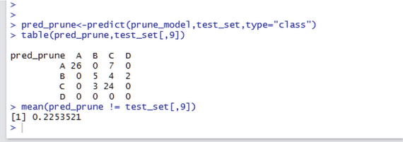
For the pruned tree, the misclassification error is 15.48 percent, and the residual mean deviance is 0.8708. The model fits better, but the misclassification error is a little higher than the full tree model. Hence, the pruned tree model did not improve the performance of the model. The next step is to carry out the process called k-fold validation. The process is as follows:
Split the data set into k folds. The suggested value is k = 10.
For each k fold in the data set, build your model on k – 1 folds and test the model to check the effectiveness for the left-out fold.
Record the prediction errors.
Repeat the steps k times so that each of the k folds are part of the test set.
The average of the error recorded in each iteration of k is called the cross-validation error, and this will be the performance metric of the model.
6.6 Summary
The chapter explained the fundamental concepts of supervised machine learning and the differences between the classification model and prediction model. You learned why the classification model also falls under prediction.
You learned the fundamentals of the probabilistic classification model using naïve Bayes. You also saw Bayes’ theorem used for classification and for predicting classes via an example in R.
This chapter described the decision-tree model, how to build the decision tree, how to select the decision tree root, and how to split the tree. You saw examples of building the decision tree, pruning the tree, and measuring the performance of the classification model.
You also learned about the bias-variance concept with respect to overfitting and underfitting.
Finally, you explored how to create a classification model, understand the measure of performance of the model, and improve the model performance, using R.