State of the Art
We are about to embark on a journey through the last five years of business forecasting literature, with over 60 selections from journals, books, whitepapers, and original contributions written just for this collection. The biggest single topic area – reflecting the intense interest from practitioners and researchers alike – is the role of artificial intelligence and machine learning in business forecasting. But traditional forecasting topics like modeling, performance evaluation, and process remain vital, and are not ignored. We've sought to include the compelling new ideas, and the divergent viewpoints, to broadly represent advances in the business forecasting profession over the past five years.
But before we begin the journey, it is worth a few moments to review and reflect upon where we are at now – business forecasting's state of the art.
* * *
FORECASTING IN SOCIAL SETTINGS: THE STATE OF THE ART*
Spyros Makridakis, Rob J. Hyndman, and Fotios Petropoulos
* * *
I. THE FACTS
A Brief History of Forecasting
In terms of human history, it is not that long since forecasting moved from the religious, the superstitious, and even the supernatural (Scott, 2015) to the more scientific. Even today, though, old fortune-telling practices still hold among people who pay to receive the “prophetic” advice of “expert” professional forecasters, including those who claim to be able to predict the stock market and make others rich by following their advice. In the emerging field of “scientific” forecasting, there is absolute certainty about two things. First, no one possesses prophetic powers, even though many pretend to do so; and, second, all predictions are uncertain: often the only thing that varies among such predictions is the extent of such uncertainty.
The field of forecasting outside the physical sciences started at the end of the nineteenth century with attempts to predict economic cycles, and continued with efforts to forecast the stock market. Later, it was extended to predictions concerning business, finance, demography, medicine, psychology, and other areas of the social sciences. The young field achieved considerable success after World War II with Robert Brown's work (Brown, 1959, 1963) on the prediction of the demand for thousands of inventory items stored in navy warehouses. Given the great variety of forecasts needed, as well as the computational requirements for doing so, the work had to be simple to carry out, using the mechanical calculators of the time. Brown's achievement was to develop various forms of exponential smoothing that were sufficiently accurate for the problems faced and computationally light. Interestingly, in the Makridakis and Hibon (1979) study and the subsequent M1 and M2 competitions, his simple, empirically-developed models were found to be more accurate than the highly sophisticated ARIMA models of Box and Jenkins (Box, Jenkins, Reinsel, and Ljung, 2015).
As computers became faster and cheaper, the field expanded, with econometricians, engineers and statisticians all proposing various advanced forecasting approaches, under the belief that a greater sophistication would improve the forecasting accuracy. There were two faulty assumptions underlying such beliefs. First, it was assumed that the model that best fitted the available data (model fit) would also be the most accurate one for forecasting beyond such data (post-sample predictions), whereas actually the effort to minimise model fit errors contributed to over-parameterisation and overfitting. Simple methods that captured the dominant features of the generating process were both less likely to overfit and likely to be at least as accurate as statistically sophisticated ones (see Pant and Starbuck, 1990). The second faulty assumption was that of constancy of patterns/relationships – assuming that the future will be an exact continuation of the past. Although history repeats itself, it never does so in precisely the same way. Simple methods tend to be affected less by changes in the data generating process, resulting in smaller post-sample errors.
Starting in the late 1960s, significant efforts were made, through empirical and other studies and competitions, to evaluate the forecasting accuracy and establish some objective findings regarding our ability to predict the future and assess the extent of the uncertainty associated with these predictions. Today, following many such studies/competitions, we have a good idea of the accuracy of the various predictions in the business, economic and social fields (and also, lately, involving climate changes), as well as of the uncertainty associated with them. Most important, we have witnessed considerable advances in the field of forecasting, which have been documented adequately in the past by two published papers. Makridakis (1986) surveyed the theoretical and practical developments in the field of forecasting and discussed the findings of empirical studies and their implications until that time. Twenty years later, Armstrong (2006) published another pioneering paper that was aimed at “summarizing what has been learned over the past quarter century about the accuracy of forecasting methods” (p. 583) while also covering new developments, including neural networks, which were in their infancy at that time. The purpose of the present paper is to provide an updated survey for non-forecasting experts who want to be informed of the state of the art of forecasting in social sciences and to understand the findings/conclusions of the M4 Competition better.
Some of the conclusions of these earlier surveys have been overturned by subsequent additional evidence. For example, Armstrong (2006) found neural nets and Box-Jenkins methods to fare poorly against alternatives, whereas now both have been shown to be competitive. For neural nets, good forecasts have been obtained when there are enormous collections of data available (Salinas, Flunkert, and Gasthaus, 2017). For Box-Jenkins methods, improved identification algorithms (Hyndman and Khandakar, 2008) have led to them being competitive with (and sometimes better than) exponential smoothing methods. Other conclusions have stood the test of time: for example, that combining forecasts improves the accuracy.
When Predictions Go Wrong
Although forecasting in the physical sciences can attain amazing levels of accuracy, such is not the case in social contexts, where practically all predictions are uncertain and a good number can be unambiguously wrong. This is particularly true when binary decisions are involved, such as the decision that faces the U.S. Federal Reserve as to whether to raise or lower interest rates, given the competing risks of inflation and unemployment. The big problem is that some wrong predictions can affect not only a firm or a small group of people, but also whole societies, such as those that involve global warming, while others may be detrimental to our health. Ioannidis, a medical professor at Stanford, has devoted his life to studying health predictions. His findings are disheartening, and were articulated in an article published in PLoS Medicine entitled “Why most published research findings are false” (Ioannidis, 2005).1 A popular piece on a similar theme in The Atlantic entitled “Lies, damned lies, and medical science” (Freedman, 2010) is less polite. It summarizes such findings as: “Much of what medical researchers conclude in their studies is misleading, exaggerated, or flat-out wrong.” Freedman concluded with the question, “why are doctors – to a striking extent – still drawing upon misinformation in their everyday practice?”
A recent case exemplifying Ioannidis' conclusions is the findings of two studies eight years apart of which the results were contradictory, making it impossible to know what advice to follow in order to benefit from medical research. In 2010, Micha, Wallace, and Mozaffarian (2010) published a meta-analysis that reviewed six studies which evaluated the effects of meat and vegetarian diets on mortality, involving a total of more than 1.5 million people. It concluded that all-cause mortality was higher for those who ate meat, mainly red or processed meat, daily. However, a new study published in 2018 (Mente and Yusuf, 2018), using a large sample of close to 220,000 people, found that eating red meat and cheese reduced cardiovascular disease by 22% and decreased the risk of early death by 25% (with such large sample sizes, all differences are statistically significant). If conflicting medical predictions, based on substantial sample sizes and with hundreds of millions of dollars having been spent on designing and conducting them, are widespread, what are we to surmise about studies in other disciplines that are less well funded, utilize small sample sizes, or base their predictions on judgment and opinion? Moreover, if the conclusions of a medical study can be reversed in a period of just eight years, how can we know that those of new studies will not produce the same contradictions? Recommendations about the treatment of disease are based on the findings of medical research, but how can such findings be trusted when, according to Ioannidis, most of them are false? Clearly, there is a predictability problem that extends beyond medicine to practically all fields of social science, including economics (Camerer et al. 2016, Dewald, Thursby, and Anderson, 1986). Fortunately, empirical studies in the field of forecasting have provided us with some objective evidence that allows us to both determine the accuracy of predictions and estimate the level of uncertainty.
There are several famous examples of forecasting errors, including Ballmer's forecast quoted earlier about the iPhone, which is possibly the most successful of all products ever marketed. In 1798, Malthus predicted that we were confronted by mass starvation, as the population was growing geometrically while food production was increasing only arithmetically. Today's material abundance and decreases in population growth in most advanced countries have been moving in the opposite direction to his predictions. In 1943, Thomas Watson, IBM's president, made his infamous prediction: “I think there is a world market for maybe five computers,” missing it by about a billion times if all computers, including smartphones, are counted (see also Schnaars, 1989). However, even recent predictions by professional organisations that specialise in forecasting, using modern computers and well-trained, PhD-holding forecasters, can go wrong, as can be seen from the complete failure of these organisations to predict the great 2007/2008 recession and its grave implications. The same has been true with technological forecasting, which failed to predict, even a few decades earlier, the arrival and widespread usage of the three major inventions of our times: the computer, the internet, and the mobile phone. Judgmental predictions have been evaluated by Tetlock (2006), who has compared the forecasts of experts in different macroeconomic fields to forecasts made by well-informed laity or those based on simple extrapolation from current trends. He concluded that not only are most experts not more accurate, but they also find it more difficult to change their minds when new evidence becomes available.
After surveying past successes and failures in forecasting, what we can conclude is that there is a significant amount of uncertainty in all of our predictions, and that such uncertainty is underestimated greatly for two reasons. First, our attitude to extrapolating in a linear fashion from the present to the future, and second, our fear of the unknown and our psychological need to reduce the anxiety associated with such a fear by believing that we can control the future by predicting it accurately (known as the illusion of control, see Langer, 1975). Thus, it becomes imperative to be aware of the difficulty of accurate predictions and the underestimation of the uncertainty associated with them, in order to be able to minimise this bias. The field of quantitative forecasting has the potential advantage that it may be possible to assess the accuracy of forecasts and the level of uncertainty surrounding them by utilising information from empirical and open forecasting competitions.
Improving Forecasting Accuracy over Time
The scientific approach to forecasting in the physical sciences began with Halley's comet predictions in the early 1700s (Halleio, 1704), which turned out to be remarkably accurate. Other forecasts followed, including the somewhat less successful meteorological forecasts of Beaufort and FitzRoy in the late 1850s (Burton, 1986). These were highly controversial at the time, and FitzRoy in particular was criticised heavily, and subsequently committed suicide. Nevertheless, he left a lasting legacy, including the word “forecast,” which he had coined for his daily weather predictions. Over the 150 years since, there has been extraordinary progress in improving the forecast accuracy not only in meteorology (Kistler et al., 2001; Saha et al., 2014) but also in other physical sciences, as the underlying physical processes have come to be understood better, the volume of observations has exploded, computing power has increased, and the ability to share information across connected networks has become available.
The social sciences are different. First, there is usually a limited theoretical or quantitative basis for representing a causal or underlying mechanism. Thus, we rely on statistical approximations that roughly describe what we observe, but may not represent a causal or underlying mechanism. Second, despite the deluge of data that is available today, much of this information does not concern what we want to forecast directly. For example, if we wish to predict the GDP next quarter, we may have an enormous amount of daily stock market data available, but no daily data on expenditures on goods and services. Third, what we are trying to forecast is often affected by the forecasts themselves. For example, central banks might forecast next year's housing price index but then raise interest rates as a result, thus leading the index to be lower than the forecast. Such feedback does not occur in astronomical or weather forecasts.
For these reasons, social science forecasts are unlikely ever to be as accurate as forecasts in the physical sciences, and the potential for improvements in accuracy is somewhat limited. Nevertheless, increases in computing power and a better understanding of how to separate signal from noise should lead to some improvements in forecast accuracy. However, this does not appear to have been the case, at least for macroeconomic forecasting (Fildes and Stekler, 2002; Heilemann and Stekler, 2013; Stekler, 2007).
On the other hand, time series forecasting has improved demonstrably over the last 30 years. We can measure the change through the published accuracies of forecasting competitions over the last 40 years, beginning with the first Makridakis competition (Makridakis et al., 1982), then the M3 competition (Makridakis and Hibon, 2000), and finally the recent M4 competition (Makridakis, Spiliotis, and Assimakopoulos, 2018a). In measuring the forecast accuracy improvement, we have applied the best-performing methods from each competition to the data from previous competitions in order to see how the methods have improved over time.
However, these comparisons are not straightforward because the forecast accuracy measures used were not consistent between competitions. In fact, there is still no agreement on the best measure of the forecast accuracy. We will therefore compare results using the MAPE (used in the first competition), the sMAPE (used in the M3 competition), and the MASE. The M4 competition used a weighted average of the sMAPE and MASE values. All measures are defined and discussed by Hyndman and Koehler (2006) and Hyndman and Athanasopoulos (2018).
In the first Makridakis competition (Makridakis et al., 1982), the best-performing method overall (as measured by MAPE) was simple exponential smoothing applied to deseasonalized data, where the deseasonalization used a classical multiplicative decomposition (Hyndman and Athanasopoulos, 2018); this is denoted by DSES. For non-seasonal data, DSES is equivalent to simple exponential smoothing.
In the M3 competition, the best method (as measured by sMAPE), and which is in the public domain, was the Theta method (Assimakopoulos and Nikolopoulos, 2000). We applied the Theta method using the thetaf() implementation from the forecast package for R (Hyndman et al., 2018), to ensure consistent application to all data sets.
In the M4 competition, the best-performing method (as measured by a weighted average of sMAPE and MASE) for which we had R code available was the FFORMA method (Montero-Manso, Athanasopoulos, Hyndman, and Talagala, 2020), which came second in the competition.
In addition to these methods, we also included, for comparison, the popular auto.arima() and ets() methods (Hyndman and Khandakar, 2008; Hyndman et al., 2002), as implemented by Hyndman et al. (2018), along with a simple average of the forecasts from these two methods (denoted “ETSARIMA”). We also include two simple benchmarks: naive and naive on the seasonally adjusted data (naive 2).
Table I.1 Comparing the Best Method from Each Forecasting Competition against Each Other and against Benchmark Methods (Thanks to Pablo Montero-Manso for providing the FFORMA forecasts for the M1 and M3 data.)
| M1 Competition | M3 Competition | M4 Competition | |||||||
|---|---|---|---|---|---|---|---|---|---|
| Method | MAPE | sMAPE | MASE | MAPE | sMAPE | MASE | MAPE | sMAPE | MASE |
| FFORMA | 15.9 | 14.4 | 1.3 | 18.4 | 12.6 | 1.1 | 14.3 | 11.8 | 1.2 |
| ETSARIMA | 17.4 | 15.3 | 1.3 | 18.7 | 13.1 | 1.1 | 14.9 | 12.3 | 1.2 |
| ETS | 17.7 | 15.6 | 1.4 | 18.7 | 13.3 | 1.2 | 15.6 | 12.8 | 1.3 |
| ARIMA | 18.9 | 16.3 | 1.4 | 19.8 | 14.0 | 1.2 | 15.2 | 12.7 | 1.2 |
| Theta | 20.3 | 16.8 | 1.4 | 17.9 | 13.1 | 1.2 | 14.7 | 12.4 | 1.3 |
| DSES | 17.0 | 15.4 | 1.5 | 19.2 | 13.9 | 1.3 | 15.2 | 12.8 | 1.4 |
| Naive 2 | 17.7 | 16.6 | 1.5 | 22.3 | 15.8 | 1.4 | 16.0 | 13.5 | 1.4 |
| Naive | 21.9 | 19.4 | 1.8 | 24.3 | 16.6 | 1.5 | 17.5 | 14.7 | 1.7 |
When we apply these methods to the data from all three competitions, we can see how the forecast accuracy has changed over time, as is shown in Table I.1. Note that the mean values of MAPE, sMAPE, and MASE have been calculated by applying the arithmetic mean across series and horizons simultaneously. Other ways of averaging the results can lead to different conclusions, due to greater weights being placed on some series or horizons. It is not always obvious from the published competition results how these calculations have been done in the past, although in the case of the M4 competition, the code has been made public to help to avoid such confusion.
There are several interesting aspects to this comparison.
- DSES did well on the M1 data and is competitive with other non-combining methods on the M3 and M4 data according to the MAPE and sMAPE, but it does poorly according to the MASE.
- While Theta did well on the M3 data (winner of that competition), it is less competitive on the M1 and M4 data.
- The most recent method (FFORMA) outperforms the other methods on every measure for the M1 and M4 competitions, and on all but the MAPE measure for the M3 competition.
- The ETSARIMA method (averaging the ETS and ARIMA forecasts) is almost as good as the FFORMA method in terms of MASE, and is easier and faster to compute.
- The results are relatively clear-cut across all competitions (in the order displayed) using the MASE criterion, but the results are less clear with the other accuracy criteria.
While there is some variation between periods, the good performances of FFORMA and ETSARIMA are relatively consistent across data sets and frequencies. Clearly, progress in forecasting methods has been uneven, but the recent M4 competition has helped to advance the field considerably in several ways, including: (1) encouraging the development of several new methods; and (2) providing a large set of data in order to allow detailed comparisons of various forecasting methods over different time granularities.
The Importance of Being Uncertain
No forecasts are exact, and so it is important to provide some measure of the forecast uncertainty. Unless such uncertainty is expressed clearly and unambiguously, forecasting is not far removed from fortune-telling.
The most general approach to expressing the uncertainty is to estimate the “forecast distribution” – the probability distribution of future observations conditional on the information available at the time of forecasting. A point forecast is usually the mean (or sometimes the median) of this distribution, and a prediction interval is usually based on the quantiles of this distribution (Hyndman and Athanasopoulos, 2018). As a consequence, forecasting has two primary tasks:
- To provide point forecasts which are as accurate as possible;
- To specify or summarise the forecast distribution.
Until relatively recently, little attention was paid to forecast distributions, or measures of the forecast distribution accuracy. For example, there was no measure of the distributional forecast uncertainty used in the M1 and M3 competitions, and it is still rare to see such measures used in Kaggle competitions.
Prediction Interval Evaluation
The simplest approach to summarising the uncertainty of a forecast distribution is to provide one or more prediction intervals with a specified probability coverage. However, it is well known that these intervals are often narrower than they should be (Hyndman et al., 2002); that is, that the actual observations fall inside the intervals less often than the nominal coverage implies. For example, the 95% prediction intervals for the ETS and ARIMA models applied to the M1 and M3 competition data, obtained using the automatic procedures in the forecast package for R, yield coverage percentages that are as low as 76.8%, and are never higher than 95%. Progress has been made in this area too, though, with the recent FFORMA method (Montero-Manso et al., 2020) providing an average coverage of 94.5% for these data sets. Figure I.1 shows the coverages for nominal 95% prediction intervals for each method and forecast horizon when applied to the M1 and M3 data. ARIMA models do particularly poorly here.
It is also evident from Figure I.1 that there are possible differences between the two data sets, with the percentage coverages being lower for the M1 competition than for the M3 competition.
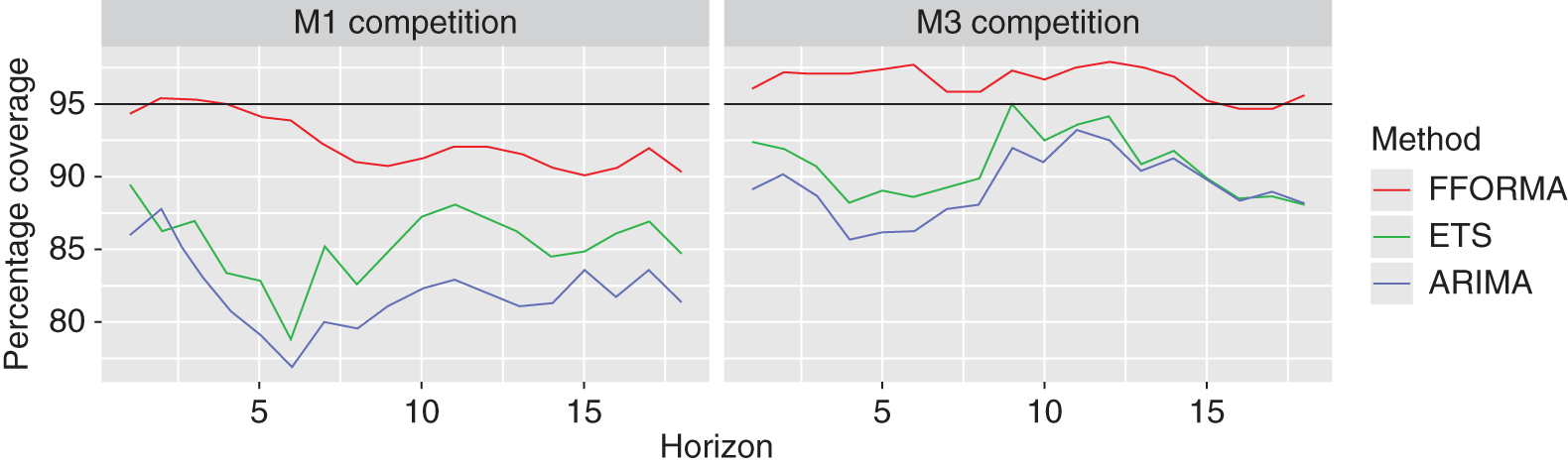
Figure I.1 Actual Coverages Achieved by Nominal 95% Prediction Intervals
There are at least three reasons for standard statistical models' underestimations of the uncertainty.
- Probably the biggest factor is that model uncertainty is not taken into account. The prediction intervals are produced under the assumption that the model is “correct,” which clearly is never the case.
- Even if the model is specified correctly, the parameters must be estimated, and also the parameter uncertainty is rarely accounted for in time series forecasting models.
- Most prediction intervals are produced under the assumption of Gaussian errors. When this assumption is not correct, the prediction interval coverage will usually be underestimated, especially when the errors have a fat-tailed distribution.
In contrast, some modern forecasting methods do not use an assumed data generating process to compute prediction intervals. Instead, the prediction intervals from FFORMA are produced using a weighted combination of the intervals from its component methods, where the weights are designed to give an appropriate coverage while also taking into account the length of the interval.
Coverage is important, but it is not the only requirement for good prediction intervals. A good prediction interval will be as small as possible while maintaining the specified coverage. Winkler proposed a scoring method for enabling comparisons between prediction intervals that takes into account both the coverage and the width of the intervals. If the 100(1−α)% prediction interval for time t is given by [lt , ut], and yt is the observation at time t, then the Winkler (1972) score is defined as the average of:
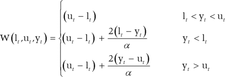
This penalises both for wide intervals (since ut − lt will be large) and for non-coverage, with observations that are well outside the interval being penalised more heavily. However, although this was proposed in 1972, it has received very little use until recently, when a scaled version of it was used in the M4 competition. The lower the score, the better the forecasts. For a discussion of some of the problems with interval scoring, see Askanazi, Diebold, Schorfheide, and Shin (2018).
Forecast Distribution Evaluation
To the best of our knowledge, the only forecasting competitions that have evaluated whole forecast distributions have been the GEFCom2014 and GEFCom2017 energy forecasting competitions (Hong et al., 2016). Both used percentile scoring as an evaluation measure.
For each time period t throughout the forecast horizon, the participants provided percentiles qi,t, where i = 1, 2, …, 99. Then, the percentile score is given by the pinball loss function:

This score is then averaged over all percentiles and all time periods in order to evaluate the full predictive density. If the observations follow the forecast distribution, then the average score will be the smallest value possible. If the observations are more spread out or deviate from the forecast distribution in some other way, then the average score will be higher. Other distribution scoring methods are also available (Gneiting and Raftery, 2007).
Without a history of forecast distribution evaluation, it is not possible to explore how this area of forecasting has improved over time. However, we recommend that future forecast evaluation studies include forecast distributions, especially in areas where the tails of the distribution are of particular interest, such as in energy and finance.
II. WHAT WE KNOW
On Explaining the Past versus Predicting the Future
Forecasting is about predicting the future, but this can only be done based on information from the past, which raises the issue of how the most appropriate information and the corresponding model for predicting the future should be selected. For a long period, and for lack of a better alternative, it was believed that such model should be chosen according to how well it could explain, that is, fit, the available past data (somewhat like asking a historian to predict the future). For instance, in the presentation of their paper to the Royal Statistical Society in London, Makridakis and Hibon (1979) had difficulty explaining their findings that single exponential smoothing was more accurate than the Box-Jenkins approach and that a combination of methods was more accurate than the individual methods being combined. Theoretically, with the correct model and assuming that the future is the same as the past, these findings would not be possible. However, this theoretical postulate does not necessarily hold, because the future could be quite different from the past. Both the superiority of combining and the higher accuracy of exponential smoothing methods relative to ARIMA models were proven again in the M1 and M2 competitions. However, some statisticians were still unwilling to accept the empirical evidence, arguing that theory was more important than empirical competitions, as was expressed powerfully by Priestley, who stated that “we must resist the temptation to read too much into the results of the analysis” (Makridakis and Hibon, 1979, p. 127).
The debate ended with the M3 Competition (Makridakis and Hibon, 2000), with its 3003 time series. Once again, the results showed the value of combining and the superior performances of some simpler methods (such as the Theta method) in comparison to other, more complicated methods (most notably one particular neural networks application). Slowly but steadily, this evidence is being accepted by a new breed of academic forecasters and well-informed practitioners who are interested in improving the accuracy of their predictions. Moreover, the accuracy of ARIMA models has improved considerably in the M3 and M4 competitions, surpassing those of exponential smoothing methods when model selection was conducted using Akaike's information criterion (Akaike, 1977).
As a result, the emphasis has shifted from arguing about the value of competitions to learning as much as possible from the empirical evidence in order to improve the theoretical and practical aspects of forecasting. The M4 Competition, which is covered in detail in this special issue, is the most recent evidence of this fundamental shift in attitudes toward forecasting and the considerable learning that has been taking place in the field. A number of academic researchers have guided this shift within universities. Determined practitioners from companies like Uber, Amazon, Google, Microsoft, and SAS, among others, present their advances every year in the International Symposium on Forecasting (ISF). They are focused on improving the forecasting accuracy and harnessing its benefits, while also being concerned about measuring the uncertainty in their predictions.
On the (Non)existence of a Best Model
Many forecasting researchers have been on a quest to identify the best forecasting model for each particular case. This quest is often viewed as the “holy grail” in forecasting. While earlier studies investigated the concept of aggregate selection (Fildes, 1989), meaning selecting one model for all series within a data set, more recent studies have suggested that such an approach can only work for highly homogeneous data sets. In fact, as Fildes and Petropoulos (2015) showed, if we had some way of identifying correctly beforehand which model would perform best for each series, we could observe savings of up to 30% compared to using the best (but same) model on all series.
Approaches for the individual selection of the best model for each series (or even for each series/horizon combination) include information criteria (Hyndman et al., 2002), validation and cross-validation approaches (Tashman, 2000), approaches that use knowledge obtained from the data to find temporary solutions to the problems faced (Fildes and Petropoulos, 2015), approaches based on time series features and expected errors (Petropoulos et al., 2014; Wang, Smith-Miles, and Hyndman, 2009), and approaches based on expert rules (Adya, Collopy, Armstrong, and Kennedy, 2001). However, all of these approaches are limited with regard to their input: they are attempting to identify the best model for the future conditional on information from the past. However, as the previous section highlighted, explaining the past is not the same as predicting the future. When dealing with real data, no well-specified “data generation processes” exist. The future might be completely different from the past, and the previous “best” models may no longer be appropriate. Even if we could identify the best model, we would be limited by the need to estimate its parameters appropriately.
In fact, there exist three types of uncertainties when dealing with real forecasting situations: model uncertainty, parameter uncertainty and data uncertainty (Petropoulos et al., 2018). In practice, such uncertainties are dealt with by combining models/methods. As George Box put it, “all models are wrong, but some are useful.” Again and again, combinations have been proved to benefit the forecasting accuracy (Clemen, 1989; Makridakis, 1989; Timmermann, 2006), while also decreasing the variance of the forecasts (Hibon and Evgeniou, 2005), thus rendering operational settings more efficient. Current approaches to forecast combinations include, among others, combinations based on information criteria (Kolassa, 2011), the use of multiple temporal aggregation levels (Andrawis et al., 2011; Athanasopoulos et al., 2017; Kourentzes et al., 2014), bootstrapping for time series forecasting (Bergmeir, Hyndman, and Benítez, 2016) and forecast pooling (Kourentzes, Barrow, and Petropoulos, 2019).
Approaches based on combinations have dominated the rankings in the latest instalment of the M competitions. It is important to highlight the fact that one element of the success of forecast combinations is the careful selection of an appropriate pool of models and their weights. One explanation for the good performance of combinations is that the design of the M competitions requires the nature and history of the series to be concealed. This reduces the amount of background information that can be applied to the forecasting problem and may give combinations an advantage relative to models that are selected individually by series. In fact, as Fildes and Petropoulos (2015) have shown, model selection can outperform forecast combinations in certain situations, such as when a dominant method exists, or under a stable environment. Finally, the evidence in the M4 results suggests that hybrid approaches, which are based on combining simple time series techniques with modern machine-learning methods at a conceptual level (rather than a forecast level), perform very well.
On the Performance of Machine Learning
The hype publicizing the considerable achievements in artificial intelligence (AI) also extends to machine learning (ML) forecasting methods. There were high expectations that hedge funds that utilized ML techniques would outperform the market (Satariano and Kumar, 2017). However, new evidence has shown that their track record is mixed, even though their potential is enormous (Asmundsson, 2018).
Although some publications have claimed to show excellent accuracies of ML forecasting methods, very often they have not been compared against sensible benchmarks. For stock-market data, for example, it is essential to include a naive benchmark, yet often this is not done (see, for example, Wang and Wang, 2017). In addition, some studies claim high levels of accuracy by hand-selecting examples where the proposed method happens to do well. Even when a reasonably large set of data is used for the empirical evaluation and the time series have not been chosen specifically to favour the proposed approach, it is essential to consider the statistical significance of any comparisons made. Otherwise, conclusions can be drawn from random noise (Pant and Starbuck, 1990).
One advantage of large forecasting competitions is that they provide a collection of data against which new methods can be tested, and for which published accuracy results are available. The data sets are also large enough that statistically significant results should be able to be achieved for any meaningful improvements in forecast accuracy.
One disadvantage is that the series are a heterogeneous mix of frequencies, lengths and categories, so that there may be some difficulty in extracting from the raw results the circumstances under which individual methods shine or fall down.
In time series forecasting, the hype has been moderated over time as studies have shown that the application of ML methods leads to poor performances in comparison to statistical methods (though some ML supporters still argue about the validity of the empirical evidence). We are neither supporters nor critics of either approach over the other, and we believe that there is considerable overlap between the statistical and ML approaches to forecasting. Moreover, they are complementary in the sense that ML methods are more vulnerable to excessive variance, while statistical ones are more vulnerable to higher bias. At the same time, the empirical evidence to date shows a clear superiority in accuracy of the statistical methods in comparison to ML ones when applied to either individual time series or large collections of heterogeneous time series. In a study using the 1045 monthly M3 series (those utilized by Ahmed, Atiya, Gayar, and El-Shishiny, 2010) that consisted of more than 81 observations, Makridakis, Spiliotis, and Assimakopoulos (2018b) found, using accepted practices to run the methods, that the most accurate ML methods were less accurate than the least accurate statistical one. Moreover, 14 of the ML methods were less accurate than naive 2.
ML methods did not do well in the M4 Competition either, with most of them doing worse than the naive 2 benchmark (for more details, see Makridakis, Spiliotis, and Assimakopoulos, 2020). We believe that it is essential to figure out the reasons for such poor performances of the ML methods. One possibility is the relatively large number of parameters associated with ML methods compared to statistical methods. Another is the number of important choices that are related to the design of ML, which are usually made using validation data, as there is no standardised ML approach. The time series used in these competitions are generally not particularly long, with a few hundred observations at most. This is simply not sufficient for building a complicated nonlinear, nonparametric forecasting model. Even if the time series are very long (at least a few thousand observations), there are difficulties with data relevance, as the dynamics of the series may have changed, and the early part of the series may bias the forecasting results.
Machine learning methods have done well in time series forecasting when forecasting an extensive collection of homogeneous data. For example, Amazon uses deep learning neural networks to predict product sales (Salinas et al., 2017; Wen et al., 2017) by exploiting their vast database of the sales histories of related products, rather than building a separate model for the sales of each product.
We expect that future research efforts will work toward making these methods more accurate. Both the best and second-best methods of the M4 Competition used ML ideas to improve the accuracy, and we would expect that additional, innovative notions would be found in the future to advance their utilization.
III. WHAT WE ARE NOT SURE ABOUT
On the Prediction of Recessions/Booms/Non-stable Environments
One area of forecasting that has attracted a considerable amount of attention is that of extreme events, which include but are not limited to economic recessions/booms and natural disasters. Such events have a significant impact from a socioeconomic perspective, but also are notoriously tricky to predict, with some being “black swans” (events with no known historical precedent).
Take as an example the great recession of 2008. At the end of December 2007, BusinessWeek reported that only 2 out of 34 forecasters predicted a recession for 2008. Even when the symptoms of the recession became more evident, Larry Kudlow (an American financial analyst and the Director of the National Economic Council under the Trump administration) insisted that there was no recession. Similarly, the Federal Open Market Committee failed to predict the 2008 recession (Stekler and Symington, 2016). Interestingly, after the recession, most economic analysts, victims of their hindsight, were able to provide detailed explanations of and reasons behind the recession, while the few “prophets” who did indeed predict the great recession were unable to offer equally good predictions for other extreme events, as if their prophetic powers had been lost overnight.
Two recent studies have taken some first steps towards predicting market crashes and bubble bursts. Gresnigt, Kole, and Franses (2015) model financial market crashes as seismic activity and create medium-term probability predictions, which consequently feed an early warning system. Franses (2016) proposes a test for identifying bubbles in time series data, as well as to indicate whether a bubble is close to bursting.
On the Performances of Humans versus Models
Judgment has always been an integral input to the forecasting process. Earlier studies focused on the comparative performances of judgmental versus statistical forecasts, when judgment was used to produce forecasts directly. However, the results of such studies have been inconclusive. For instance, while Lawrence, Edmundson, and O'Connor (1985) and Makridakis et al. (1993) found that unaided human judgment can be as good as the best statistical methods from the M1 forecasting competition, Carbone and Gorr (1985) and Sanders (1992) found judgmental point forecasts to be less accurate than statistical methods. The reason for these results is the fact that well-known biases govern judgmental forecasts, such as the tendency of forecasters to dampen trends (Lawrence et al., 2006; Lawrence and Makridakis, 1989), as well as anchoring and adjustment (O'Connor, Remus, and Griggs, 1993) and the confusion of the signal with noise (Harvey, 1995; Reimers and Harvey, 2011). On the other hand, statistical methods are consistent and can handle vast numbers of time series seamlessly. Still, judgment is the only option for producing estimates for the future when data are not available.
Judgmental biases apply even to forecasters with domain or technical expertise. As such, the expert knowledge elicitation (EKE; Bolger and Wright, 2017) literature has examined many ways of designing methods so as to reduce the danger of biased judgments from experts. Strategies for mitigating humans' biases include decomposing the task (Edmundson, 1990; Webby, O'Connor, and Edmundson, 2005), offering alternative representations (tabular versus graphical formats; see Harvey and Bolger, 1996) and providing feedback (Petropoulos, Goodwin, and Fildes, 2017).
The previous discussion has focused on judgmental forecasts that are produced directly. However, the judgment in forecasting can also be applied in the form of interventions (adjustments) to the statistical forecasts that are produced by a forecasting support system. Model-based forecasts are adjusted by experts frequently in operations/supply chain settings (Fildes et al., 2009, Franses and Legerstee, 2010). Such revised forecasts often differ significantly from the statistical ones (Franses and Legerstee, 2009); however, small adjustments are also observed, and are linked with a sense of ownership of the forecasters (Fildes et al., 2009). Experts tend to adjust upwards more often than downwards (Franses and Legerstee, 2010), which can be attributed to an optimism bias (Trapero, Pedregal, Fildes, and Kourentzes, 2013), but such upwards adjustments are far less effective (Fildes et al., 2009). The empirical evidence also suggests that experts can reduce the forecasting error when the adjustment size is not too large (Trapero et al., 2013).
Another point in the forecasting process at which judgment can be applied is that of model selection. Assuming that modern forecasting software systems offer many alternative models, managers often rely on their judgment in order to select the most suitable one, rather than pushing the magic button labelled “automatic selection” (which selects between models based on algorithmic/statistical approaches, for example, using an information criterion). The study by Petropoulos et al. (2018) is the first to offer some empirical evidence on the performance of judgmental versus algorithmic selection. When the task follows a decomposition approach (selection of the applicable time series patterns, which is then translated to the selection of the respective forecasting model), on average the judgmental selection is as good as selecting via statistics, while humans more often have the advantage of avoiding the worst of the candidate models.
Two strategies are particularly useful for enhancing the judgmental forecasting performance. The first strategy is a combination of statistics and judgment (Blattberg and Hoch, 1990). This can be applied intuitively to cases where statistical and judgmental forecasts have been produced independently, but it works even in cases where the managerial input could be affected by the model output, as in judgmental adjustments. Several studies have shown that adjusting the adjustments can lead not only to an improved forecasting performance (Fildes et al., 2009; Franses and Legerstee, 2011), but also to a better inventory performance (Wang and Petropoulos, 2016). The second strategy is the mathematical aggregation of the individual judgments that have been produced independently, also known as the “wisdom of crowds” (Surowiecki, 2005). In Petropoulos, Kourentzes, Nikolopoulos, and Siemsen's (2018) study of model selection, the aggregation of the selections of five individuals led to a forecasting performance that was significantly superior to that of algorithmic selection.
In summary, we observe that, over time, the research focus has shifted from producing judgmental forecasts directly to adjusting statistical forecasts and selecting between forecasts judgmentally. The value added to the forecasting process by judgment increases as we shift further from merely producing a forecast judgmentally.
However, given the exponential increase in the number of series that need to be forecast by a modern organisation (for instance, the number of stock-keeping units in a large retailer may very well exceed 100,000), it is not always either possible or practical to allocate the resources required to manage each series manually.
On the Value of Explanatory Variables
The use of exogenous explanatory variables would seem an obvious way of improving the forecast accuracy. That is, rather than relying only on the history of the series that we wish to forecast, we can utilise other relevant and available information as well.
In some circumstances, the data from explanatory variables can improve the forecast accuracy significantly. One such situation is electricity demand forecasting, where current and past temperatures can be used as explanatory variables (Ben Taieb and Hyndman, 2014). The electricity demand is highly sensitive to the ambient temperature, with hot days leading to the use of air-conditioning and cold days leading to the use of heating. Mild days (with temperatures around 20 °C) tend to have the lowest electricity demand.
However, often the use of explanatory variables is not as helpful as one might imagine. First, the explanatory variables themselves may need to be forecast. In the case of temperatures, good forecasts are available from meteorological services up to a few days ahead, and these can be used to help forecast the electricity demand. However, in many other cases, forecasting the explanatory variables may be just as difficult as forecasting the variable of interest. For example, Ashley (1988) argues that the forecasts of many macroeconomic variables are so inaccurate that they should not be used as explanatory variables. Ma, Fildes, and Huang (2016) demonstrate that including competitive promotional variables as explanatory variables for retail sales is of limited value, but that adding focal variables leads to substantial improvements over time series modelling with promotional adjustments.
A second problem arises due to the assumption that the relationships between the forecast variable and the explanatory variables will continue. When this assumption breaks down, we face model misspecification.
A third issue is that the relationship between the forecast variable and the explanatory variables needs to be strong and estimated precisely (Brodie, Danaher, Kumar, and Leeflang, 2001). If the relationship is weak, there is little value in including the explanatory variables in the model.
It is possible to assess the value of explanatory variables and to test whether either of these problems is prevalent by comparing the forecasts from three separate approaches: (1) a purely time series approach, ignoring any information that may be available in explanatory variables; (2) an ex-post forecast, building a model using explanatory variables but then using the future values of those variables when producing an estimate; and (3) an ex-ante forecast, using the same model but substituting the explanatory variables with their forecasts.
Athanasopoulos, Hyndman, Song, and Wu (2011) carried out this comparison in the context of tourism data, as part of the 2010 tourism forecasting competition. In their case, the explanatory variables included the relative CPI and prices between the source and destination countries. Not only were the purely time series forecasts better than the models that included explanatory variables, but also the ex-ante forecasts were better than the ex-post forecasts. This suggests that the relationships between tourism numbers and the explanatory variables changed over the course of the study. Further supporting this conclusion is the fact that time-varying parameter models did better than fixed parameter models. However, the time-varying parameter models did not do as well as the purely time series models, showing that the forecasts of the explanatory variables were also problematic.
To summarise, explanatory variables can be useful, but only under two specific conditions: (1) when there are accurate forecasts of the explanatory variables available; and (2) when the relationships between the forecasts and the explanatory variables are likely to continue into the forecast period. Both conditions are satisfied for electricity demand, but neither condition is satisfied for tourism demand. Unless both conditions are satisfied, time series forecasting methods are better than using explanatory variables.
IV. WHAT WE DON'T KNOW
On Thin/Fat Tails and Black Swans
Another misconception that prevailed in statistical education for a long time was that normal distributions could approximate practically all outcomes/events, including the errors of statistical models. Furthermore, there was little or no discussion of what could be done when normality could not be assured. Now, it is accepted that Gaussian distributions, although extremely useful, are of limited value for approximating some areas of application (Cooke, Nieboer, and Misiewicz, 2014; Makridakis and Taleb, 2009), and in particular those that refer to forecast error distributions, describing the uncertainty in forecasting. This paper has emphasized the critical role of uncertainty and expressed our conviction that providing forecasts without specifying the levels of uncertainty associated with them amounts to nothing more than fortune-telling. However, it is one thing to identify uncertainty, but quite another to get prepared to face it realistically and effectively. Furthermore, it must be clear that it is not possible to deal with uncertainty without either incurring a cost or accepting lower opportunity benefits.
Table I.2 distinguishes four types of events, following Rumsfeld's classification. In Quadrant I, the known/knowns category, the forecasting accuracy depends on the variance (randomness) of the data, and can be assessed from past information. Moreover, the uncertainty is well defined and can be measured, usually following a normal distribution with thin tails. In Quadrant II (known/unknowns), which includes events like recessions, the accuracy of forecasting cannot be assessed, as the timing of a recession, crisis or boom cannot be known and their consequences can vary widely from one recession to another. The uncertainty in this quadrant is considerably greater, while its implications are much harder to assess than those in Quadrant I. It is characterized by fat tails, extending well beyond the three sigmas of the normal curve. A considerable problem that amplifies the level of uncertainty is that, during a recession, a forecast, such as the sales of a product, moves from Quadrant I to Quadrant II, which increases the uncertainty considerably and makes it much harder to prepare to face it.
Things can get still more uncertain in Quadrant III, for two reasons. First, judgmental biases influence events; for instance, people fail to address obviously high-impact dangers before they spiral out of control (Wucker, 2016). Second, it is not possible to predict the implications of self-fulfilling and self-defeating prophecies for the actions and reactions of market players. This category includes strategy and other important decisions where the forecast or the anticipation of an action or plan can modify the future course of events, mainly when there is a zero-sum game where the pie is fixed. Finally, in Quadrant IV, any form of forecasting is difficult by definition, requiring the analysis and evaluation of past data to determine the extent of the uncertainty and risk involved. Taleb, the author of Black Swan (Taleb, 2007), is more pessimistic, stating that the only way to be prepared to face black swans is by having established antifragile strategies that would allow one to dampen the negative consequences of any black swans that may appear. Although other writers have suggested insurance and robust strategies for coping with uncertainty and risk, Taleb's work has brought renewed attention to the issue of highly improbable, high-stakes events and has contributed to making people aware of the need to be prepared to face them, such as, for instance, having enough cash reserves to survive a significant financial crisis like that of 2007–2008 or having invested in an adequate capacity to handle a boom.
Table I.2 Accuracy of Forecasting, Type of Uncertainty, and Extent of Risk
| Uncertainty | Known | I. Known/known (Law of large numbers, independent events, e.g. sales of toothbrushes, shoes or beer) Forecasting: Accurate (depending on variance) Uncertainty: Thin-tailed and measurable Risks: Manageable, can be minimized |
III. Unknown/known (Cognitive biases, strategic moves, e.g. Uber reintroducing AVs in a super-competitive industry) Forecasting: Accuracy depends on several factors Uncertainty: Extensive and hard to measure Risk: Depends on the extent of biases, strategy success |
| Unknown | II. Known/unknown (Unusual/special conditions, e.g. the effects of the 2007/2008 recession on the economy) Forecasting: Inaccuracy can vary considerably Uncertainty: Fat-tailed, hard to measure Risks: Can be substantial, tough to manage |
IV. Unknown/unknown (Black swans: Low-probability, high-impact events, e.g. the implications of a total collapse in global trade) Forecasting: Impossible Uncertainty: Unmeasurable Risks: Unmanageable except through costly antifragile strategies | |
| Known | Unknown | ||
| Forecast Events | |||
What needs to be emphasised is that dealing with any uncertainty involves a cost. The uncertainty that the sales forecast may be below the actual demand can be dealt with by keeping enough inventories, thus avoiding the risk of losing customers. However, such inventories cost money to keep and require warehouses in which to be stored. In other cases, the uncertainty that a share price may decrease can be dealt with through diversification, buying baskets of stocks, thereby reducing the chance of large losses; however, one then foregoes profits when individual shares increase more than the average. Similarly, antifragile actions such as keeping extra cash for unexpected crises also involve opportunity costs, as such cash could instead have been invested in productive areas to increase income and/or reduce costs and increase profits.
The big challenge, eloquently expressed by Bertrand Russell, is that we need to learn to live without the support of comforting fairy tales; he also added that it is perhaps the chief achievement of philosophy “to teach us how to live without certainty, and yet without being paralysed by hesitation.” An investor should not stop investing merely because of the risks involved.
On Causality
Since the early years, humans have always been trying to answer the “why” question: what are the causal forces behind an observed result. Estimating the statistical correlation between two variables tells us little about the cause–effect relationship between them. Their association may be due to a lurking (extraneous) variable, unknown forces, or even chance. In the real world, there are just too many intervening, confounding and mediating variables, and it is hard to assess their impacts using traditional statistical methods. Randomised controlled trials (RCTs) have been long considered the “gold standard” in designing scientific experiments for clinical trials. However, as with every laboratory experiment, RCTs are limited in the sense that, in most cases, the subjects are not observed in their natural environment (medical trials may be an exception). Furthermore, RCTs may be quite impossible in cases such as the comparison of two national economic policies.
An important step towards defining causality was taken by Granger (1969), who proposed a statistical test for determining whether the (lagged) values of one time series can be used for predicting the values of another series. Even if it is argued that Granger causality only identifies predictive causality (the ability to predict one series based on another series), not true causality, it can still be used to identify useful predictors, such as promotions as explanatory variables for future sales.
Structural equation models (SEMs) have also been being used for a long time for modelling the causal relationships between variables and for assessing unobservable constructs. However, the linear-in-nature SEMs make assumptions with regard to the model form (which variables are included in the equations) and the distribution of the error. Pearl (2000) extends SEMs from linear to nonparametric, which allows the total effect to be estimated without any explicit modelling assumptions. Pearl and Mackenzie (2018) describe how we can now answer questions about ‘how' or ‘what if I do' (intervention) and ‘why' or ‘what if I had done' (counterfactuals). Two tools have been instrumental in these developments. One is a qualitative depiction of the model that includes the assumptions and relationships among the variables of interest; such graphical depictions are called causal diagrams (Pearl, 1995). The second is the development of the causal calculus that allows for interventions by modifying a set of functions in the model (Huang and Valtorta, 2012; Pearl, 1993; Shpitser and Pearl, 2006). These tools provide the means of dealing with situations in which confounders and/or mediators would render the methods of traditional statistics and probabilities impossible. The theoretical developments of Pearl and his colleagues are yet to be evaluated empirically.
On Luck (and Other Factors) versus Skills
A few lucky investing decisions are usually sufficient for stock-pickers to come to be regarded as stock market gurus. Similarly, a notoriously bad weather, economic or political forecast is sometimes sufficient to destroy the career of an established professional. Unfortunately, the human mind tends to focus on the salient and vibrant pieces of information that make a story more interesting and compelling. In such cases, we should always keep in mind that eventually “expert” stock-pickers' luck will run out. Similarly, a single inaccurate forecast does not make one a bad forecaster. Regression to the mean has taught us that an excellent landing for pilot trainees is usually followed by a worse one, and vice versa. The same applies to the accuracy of forecasts.
Regardless of the convincing evidence of regression to the mean, we humans tend to attribute successes to our abilities and skills, but failures to bad luck. Moreover, in the event of failures, we are very skillful at inventing stories, theories and explanations for what went wrong and why we did actually know what would have happened (hindsight bias). The negative relationship between actual skill/expertise and beliefs in our abilities has also been examined extensively, and is termed the Dunning-Kruger effect: the least-skilled people tend to over-rate their abilities.
Tetlock, Gardner, and Richards (2015), in their Superforecasting book, enlist the qualities of “superforecasters” (individuals that consistently have higher skill/luck ratios than regular forecasters). Such qualities include, among others, a 360° “dragonfly” view, balancing under- and overreacting to information, balancing under- and overconfidence, searching for causal forces, decomposing the problem into smaller, more manageable ones, and looking back to evaluate objectively what has happened. However, even superstars are allowed to have a bad day from time to time.
If we are in a position to provide our forecasters with the right tools and we allow them to learn from their mistakes, then their skills will improve over time. We need to convince companies not to operate under a one-big-mistake-and-you're-out policy (Goodwin, 2017). The performances of forecasters should be tracked and monitored over time and should be compared to those of other forecasts, either statistical or judgmental. Also, linking motivation with an improved accuracy directly could aid the forecast accuracy further (Fildes et al., 2009); regardless of how intuitive this argument might be, there are plenty of companies that still operate with motivational schemes that directly contradict the need for accuracy, as is the case where bonuses are given to salesmen who have exceeded their forecasts.
Goodwin (2017) suggests that, instead of evaluating the outcomes of forecasts based solely on their resulting accuracies, we should turn our attention to evaluating the forecasting process that was used to produce the forecasts in the first place. This is particularly useful when evaluating forecasts over time is either not feasible or impractical, as is the case with one-off forecasts such as the introduction of a significant new product. In any case, even if the forecasting process is designed and implemented appropriately, we should still expect the forecasts to be ‘off' in about 1 instance out of 20 assuming 95% prediction intervals, a scenario which is not that remote.
V. CONCLUSIONS
Although forecasting in the hard sciences can attain remarkable levels of accuracy, such is not the case in the social domains, where large errors are possible and all predictions are uncertain. Forecasts are indispensable for decisions of which the success depends a good deal on the accuracy of these forecasts. This paper provides a survey of the state of the art of forecasting in social sciences that is aimed at non-forecasting experts who want to be informed on the latest developments in the field, and possibly to figure out how to improve the accuracy of their own predictions.
Over time, forecasting has moved from the domains of the religious and the superstitious to that of the scientific, accumulating concrete knowledge that is then used to improve its theoretical foundation and increase its practical value. The outcome has been enhancements in forecast accuracy and improvements in estimating the uncertainty of its predictions. A major contributor to the advancement of the field has been the empirical studies that have provided objective evidence for comparing the accuracies of the various methods and validating different hypotheses. Despite all its challenges, forecasting for social settings has improved a lot over the years.
Our discussions above suggest that more progress needs to be made in forecasting under uncertain conditions, such as unstable economic environments or when fat tails are present. Also, despite the significant advances that have been achieved in research around judgment, there are still many open questions, such as the conditions under which judgment is most likely to outperform statistical models and how to minimise the negative effects of judgmental heuristics and biases. More empirical studies are needed to better understand the added value of collecting data on exogenous variables and the domains in which their inclusion in forecasting models is likely to provide practical improvements in forecasting performances. Another research area that requires rigorous empirical investigation is that of causality, and the corresponding theoretical developments.
These are areas that future forecasting competitions can focus on. We would like to see future competitions include live forecasting tasks for high-profile economic series. We would also like to see more competitions exploring the value of exogenous variables. Competitions focusing on specific domains are also very important. In the past, we have seen competitions on neural networks (Crone, Hibon, and Nikolopoulos, 2011), tourism demand (Athanasopoulos et al., 2011) and energy (Hong, Pinson, and Fan, 2014; Hong et al., 2016; Hong, Xie, and Black, 2019); we would also like to see competitions that focus on intermittent demand and retailing, among others. Furthermore, it would be great to see more work done on forecasting one-off events, in line with the Good Judgment2 project. Last but not least, we need a better understanding of how improvements in forecast accuracy translate into ‘profit,' and how to measure the cost of forecast errors.
NOTES
- 1. Ioannidis' paper is one of the most viewed/downloaded papers published in PLoS, with more than 2.3 million views and more than 350K downloads.
- 2. www.gjopen.com/.
REFERENCES
- Adya, M., Collopy, F., Armstrong, J. S., and Kennedy, M. (2001). Automatic identification of time series features for rule-based forecasting. International Journal of Forecasting 17 (2): 143–157.
- Ahmed, N. K., Atiya, A. F., Gayar, N. E., and El-Shishiny, H. (2010). An empirical comparison of machine learning models for time series forecasting. Econometric Reviews 29 (5–6): 594–621.
- Akaike, H. (1977). On entropy maximization principle. In: Application of Statistics (pp. 27–41). North-Holland Publishing Company.
- Andrawis, R. R., Atiya, A. F., and El-Shishiny, H. (2011). Combination of long-term and short-term forecasts, with application to tourism demand forecasting. International Journal of Forecasting 27 (3): 870–886.
- Armstrong, J. S. (2006). Findings from evidence-based forecasting: Methods for reducing forecast error. International Journal of Forecasting 22 (3): 583–598.
- Ashley, R. (1988). On the relative worth of recent macroeconomic forecasts. International Journal of Forecasting 4 (3): 363–376.
- Askanazi, R., Diebold, F. X., Schorfheide, F., and Shin, M. (2018). On the comparison of interval forecasts. https://www.sas.upenn.edu/fdiebold/papers2/Eval.pdf
- Asmundsson, J. (2018). The big problem with machine learning algorithms. Bloomberg News. https://www.bloomberg.com/news/articles/2018-10-09/the-big-problem-with-machine-learning-algorithms
- Assimakopoulos, V., and Nikolopoulos, K. (2000). The theta model: A decomposition approach to forecasting. International Journal of Forecasting 16 (4): 521–530.
- Athanasopoulos, G., Hyndman, R. J., Kourentzes, N., and Petropoulos, F. (2017). Forecasting with temporal hierarchies. European Journal of Operational Research 262 (1): 60–74.
- Athanasopoulos, G., Hyndman, R. J., Song, H., and Wu, D. C. (2011). The tourism forecasting competition. International Journal of Forecasting 27 (3): 822–844.
- Ben Taieb, S., and Hyndman, R. J. (2014). A gradient boosting approach to the Kaggle load forecasting competition. International Journal of Forecasting 30 (2): 382–394.
- Bergmeir, C., Hyndman, R. J., and Benítez, J. M. (2016). Bagging exponential smoothing methods using STL decomposition and Box–Cox transformation. International Journal of Forecasting 32 (2): 303–312.
- Blattberg, R. C., and Hoch, S. J. (1990). Database models and managerial intuition: 50% model + 50% manager. Management Science 36 (8): 887–899.
- Bolger, F., and Wright, G. (2017). Use of expert knowledge to anticipate the future: Issues, analysis and directions. International Journal of Forecasting 33 (1): 230–243.
- Box, G. E. P., Jenkins, G. M., Reinsel, G. C., and Ljung, G. M. (2015). Time series analysis: Forecasting and control (5th ed.). Wiley.
- Brodie, R. J., Danaher, P. J., Kumar, V., and Leeflang, P. S. H. (2001). Econometric models for forecasting market share. In J. S. Armstrong (Ed.), Principles of forecasting: A handbook for researchers and practitioners (pp. 597–611). Springer US.
- Brown, R. G. (1959). Statistical forecasting for inventory control. McGraw-Hill.
- Brown, R. G. (1963). Smoothing, forecasting and prediction of discrete time series. Courier Corporation.
- Burton, J. (1986). Robert FitzRoy and the early history of the Meteorological Office. British Journal for the History of Science 19 (2): 147–176.
- Camerer, C. F., Dreber, A., Forsell, E., et al. (2016). Evaluating replicability of laboratory experiments in economics. Science 351 (6280): 1433–1436.
- Carbone, R., and Gorr, W. L. (1985). Accuracy of judgmental forecasting of time series. Decision Sciences 16 (2): 153–160.
- Clemen, R. T. (1989). Combining forecasts: A review and annotated bibliography. International Journal of Forecasting 5 (4): 559–583.
- Cooke, R. M., Nieboer, D., and Misiewicz, J. (2014). Fat-tailed distributions: data, diagnostics and dependence. Wiley.
- Crone, S. F., Hibon, M., and Nikolopoulos, K. (2011). Advances in forecasting with neural networks? Empirical evidence from the NN3 competition on time series prediction. International Journal of Forecasting 27 (3): 635–660.
- Dewald, W. G., Thursby, J. G., and Anderson, R. G. (1986). Replication in empirical economics: The Journal of Money, Credit and Banking project. The American Economic Review 76 (4): 587–603.
- Edmundson, R. H. (1990). Decomposition; a strategy for judgemental forecasting. Journal of Forecasting 9 (4): 305–314.
- Fildes, R. (1989). Evaluation of aggregate and individual forecast method selection rules. Management Science 35 (9): 1056–1065.
- Fildes, R., Goodwin, P., Lawrence, M., and Nikolopoulos, K. (2009). Effective forecasting and judgmental adjustments: An empirical evaluation and strategies for improvement in supply-chain planning. International Journal of Forecasting 25 (1): 3–23.
- Fildes, R., and Petropoulos, F. (2015). Simple versus complex selection rules for forecasting many time series. Journal of Business Research 68 (8): 1692–1701.
- Fildes, R., and Stekler, H. (2002). The state of macroeconomic forecasting. Journal of Macroeconomics 24 (4): 435–468.
- Franses, P. H. (2016). A simple test for a bubble based on growth and acceleration. Computational Statistics & Data Analysis 100, 160–169.
- Franses, P. H., and Legerstee, R. (2009). Properties of expert adjustments on model-based SKU-level forecasts. International Journal of Forecasting 25 (1): 35–47.
- Franses, P. H., and Legerstee, R. (2010). Do experts' adjustments on model-based SKU-level forecasts improve forecast quality? Journal of Forecasting 29 (3): 331–340.
- Franses, P. H., and Legerstee, R. (2011). Combining SKU-level sales forecasts from models and experts. Expert Systems with Applications 38 (3): 2365–2370.
- Freedman, D. H. (2010, November). Lies, damned lies, and medical science. The Atlantic. https://www.theatlantic.com/magazine/archive/2010/11/lies-damned-lies-and-medical-science/308269/
- Gneiting, T., and Raftery, A. E. (2007). Strictly proper scoring rules, prediction, and estimation. Journal of the American Statistical Association 102 (477): 359–378.
- Goodwin, P. (2017). Forewarned: A sceptic's guide to prediction. Biteback Publishing.
- Granger, C. W. J. (1969). Investigating causal relations by econometric models and cross-spectral methods. Econometrica 37 (3): 424–438.
- Gresnigt, F., Kole, E., and Franses, P. H. (2015). Interpreting financial market crashes as earthquakes: A new early warning system for medium term crashes. Journal of Banking & Finance 56, 123–139.
- Halleio, E. (1704). Astronomiae cometicae synopsis, Autore Edmundo Halleio apud Oxonienses. Geometriae Professore Saviliano, & Reg. Soc. S. Philosophical Transactions of the Royal Society of London Series I 24, 1882–1899.
- Harvey, N. (1995). Why are judgments less consistent in less predictable task situations? Organizational Behavior and Human Decision Processes 63 (3): 247–263.
- Harvey, N., and Bolger, F. (1996). Graphs versus tables: Effects of data presentation format on judgemental forecasting. International Journal of Forecasting 12 (1): 119–137.
- Heilemann, U., and Stekler, H. O. (2013). Has the accuracy of macroeconomic forecasts for Germany improved? German Economic Review 14 (2): 235–253.
- Hibon, M., and Evgeniou, T. (2005). To combine or not to combine: Selecting among forecasts and their combinations. International Journal of Forecasting 21, 15–24.
- Hong, T., Pinson, P., and Fan S. (2014). Global energy forecasting competition 2012. International Journal of Forecasting 30 (2): 357–363.
- Hong, T., Pinson, P., Fan, S., et al. (2016). Probabilistic energy forecasting: Global energy forecasting competition 2014 and beyond. International Journal of Forecasting 32 (3): 896–913.
- Hong, T., Xie, J., and Black, J. (2019). Global energy forecasting competition 2017: Hierarchical probabilistic load forecasting. International Journal of Forecasting 35(4): 1389–1399.
- Huang, Y., and Valtorta, M. (2012). Pearl's calculus of intervention is complete. arXiv preprint arXiv: 1206.6831.
- Hyndman, R. J., and Athanasopoulos, G. (2018). Forecasting: Principles and practice (2nd ed.), OTexts.
- Hyndman, R., Athanasopoulos, G., Bergmeir, C., et al. (2018). Forecast: Forecasting functions for time series and linear models. http://pkg.robjhyndman.com/forecast
- Hyndman, R. J., and Khandakar, Y. (2008). Automatic time series forecasting: The forecast package for R. Journal of Statistical Software 27 (3): 1–22.
- Hyndman, R. J., and Koehler, A. B. (2006). Another look at measures of forecast accuracy. International Journal of Forecasting 22 (4): 679–688.
- Hyndman, R. J., Koehler, A. B., Snyder, R. D., and Grose, S. (2002). A state space framework for automatic forecasting using exponential smoothing methods. International Journal of Forecasting 18 (3): 439–454.
- Ioannidis, J. P. A. (2005). Why most published research findings are false. PLoS Medicine 2 (8): Article e124.
- Kistler, R., Kalnay, E., Collins, W., et al. (2001). The NCEP–NCAR 50-year reanalysis: Monthly means CD-ROM and documentation. Bulletin of the American Meteorological Society 82 (2): 247–268.
- Kolassa, S. (2011). Combining exponential smoothing forecasts using akaike weights. International Journal of Forecasting 27 (2): 238–251.
- Kourentzes, N., Barrow, D., and Petropoulos, F. (2019). Another look at forecast selection and combination: Evidence from forecast pooling. International Journal of Production Economics 209, 226–235.
- Kourentzes, N., Petropoulos, F., and Trapero, J. R. (2014). Improving forecasting by estimating time series structural components across multiple frequencies. International Journal of Forecasting 30 (2): 291–302.
- Langer, E. J. (1975). The illusion of control. Journal of Personality and Social Psychology 32 (2): 311–328.
- Lawrence, M. J., Edmundson, R. H., and O'Connor, M. J. (1985). An examination of the accuracy of judgmental extrapolation of time series. International Journal of Forecasting 1 (1): 25–35.
- Lawrence, M., Goodwin, P., O'Connor, M., and Önkal, D. (2006). Judgmental forecasting: A review of progress over the last 25 years. International Journal of Forecasting 22 (3): 493–518.
- Lawrence, M., and Makridakis, S. (1989). Factors affecting judgmental forecasts and confidence intervals. Organizational Behavior and Human Decision Processes 43 (2): 172–187.
- Ma, S., Fildes, R., and Huang, T. (2016). Demand forecasting with high dimensional data: The case of SKU retail sales forecasting with intra- and inter-category promotional information. European Journal of Operational Research 249 (1): 245–257.
- Makridakis, S. (1986). The art and science of forecasting: An assessment and future directions. International Journal of Forecasting 2 (1): 15–39.
- Makridakis, S. (1989). Why combining works? International Journal of Forecasting 5 (4): 601–603.
- Makridakis, S., Andersen, A., Carbone, R., et al. (1982). The accuracy of extrapolation (time series) methods: Results of a forecasting competition. Journal of Forecasting 1 (2): 111–153.
- Makridakis, S., Chatfield, C., Hibon, M., et al. (1993). The M2-competition: A real-time judgmentally based forecasting study. International Journal of Forecasting 9 (1): 5–22.
- Makridakis, S., and Hibon, M. (1979). Accuracy of forecasting: An empirical investigation. Journal of the Royal Statistical Society, Series A 142 (2): 97–145.
- Makridakis, S., and Hibon, M. (2000). The M3 competition: Results, conclusions, and implications. International Journal of Forecasting 16 (4): 451–476.
- Makridakis, S., Spiliotis, E., and Assimakopoulos, V. (2018a). The M4 competition: Results, findings, conclusion and way forward. International Journal of Forecasting 34 (4): 802–808.
- Makridakis, S., Spiliotis, E., and Assimakopoulos, V. (2018b). Statistical and machine learning forecasting methods: Concerns and ways forward. PloS One 13 (3): Article e0194889.
- Makridakis, S., Spiliotis, E., and Assimakopoulos, V. (2020). The M4 competition: 100,000 time series and 61 forecasting methods. International Journal of Forecasting 36 (1): 54–74.
- Makridakis, S., and Taleb, N. (2009). Decision making and planning under low levels of predictability. International Journal of Forecasting 25 (4): 716–733.
- Mente, A., and Yusuf, S. (2018). Evolving evidence about diet and health. The Lancet Public Health 3 (9): e408–e409.
- Micha, R., Wallace, S. K., and Mozaffarian, D. (2010). Red and processed meat consumption and risk of incident coronary heart disease, stroke, and diabetes mellitus: A systematic review and meta-analysis. Circulation 121 (21): 2271–2283.
- Montero-Manso, P., Athanasopoulos, G., Hyndman, R. J., and Talagala, T. S. (2020). FFORMA: Feature-based forecast model averaging. International Journal of Forecasting 36 (1): 86–92.
- O'Connor, M., Remus, W., and Griggs, K. (1993). Judgmental forecasting in times of change. International Journal of Forecasting 9 (2): 163–172.
- Pant, P. N., and Starbuck, W. H. (1990). Innocents in the forest: Forecasting and research methods. Journal of Management 16 (2): 433–460.
- Pearl, J. (1993). Comment: Graphical models, causality and intervention. Statistical Science 8 (3): 266–269.
- Pearl, J. (1995). Causal diagrams for empirical research. Biometrika 82 (4): 669–688.
- Pearl, J. (2000). Causality: Models, reasoning, and inference. Cambridge University Press.
- Pearl, J., and Mackenzie D. (2018). The book of why: The new science of cause and effect. Allen Lane.
- Petropoulos F., Goodwin P., and Fildes, R. (2017). Using a rolling training approach to improve judgmental extrapolations elicited from forecasters with technical knowledge. International Journal of Forecasting 33 (1): 314–324.
- Petropoulos F., Hyndman, R. J., and Bergmeir, C. (2018a). Exploring the sources of uncertainty: Why does bagging for time series forecasting work? European Journal of Operational Research 268 (2): 545–554.
- Petropoulos, F., Kourentzes, N., Nikolopoulos, K., and Siemsen, E. (2018b). Judgmental selection of forecasting models. Journal of Operations Management 60: 34–46.
- Petropoulos, F., Makridakis, S., Assimakopoulos, V., and Nikolopoulos, K. (2014). ‘Horses for courses’ in demand forecasting. European Journal of Operational Research 237, 152–163.
- Reimers, S., and Harvey, N. (2011). Sensitivity to autocorrelation in judgmental time series forecasting. International Journal of Forecasting 27 (4): 1196–1214.
- Saha, S., Moorthi, S., Wu, X., et al. (2014). The NCEP climate forecast system, version 2. Journal of Climate 27 (6): 2185–2208.
- Salinas, D., Flunkert, V., and Gasthaus, J. (2017). DeepAR: Probabilistic forecasting with autoregressive recurrent networks. arXiv preprint arXiv: 1704.04110.
- Sanders, N. R. (1992). Accuracy of judgmental forecasts: A comparison. Omega 20 (3): 353–364.
- Satariano, A., and Kumar, N. (2017). The massive hedge fund betting on AI. Bloomberg News. https://www.bloomberg.com/news/features/2017-09-27/the-massive-hedge-fund-betting-on-ai
- Schnaars, S. P. (1989). Megamistakes: Forecasting and the myth of rapid technological change (29th ed.). The Free Press.
- Scott, M. (2015). Delphi: A history of the center of the ancient world. Princeton University Press.
- Shpitser, I., and Pearl, J. (2006). Identification of conditional interventional distributions. In: Proceedings of the 22nd Conference on Uncertainty in Artificial Intelligence (pp. 437–444). UAI 2006.
- Stekler, H. O. (2007). The future of macroeconomic forecasting: Understanding the forecasting process. International Journal of Forecasting 23 (2): 237–248.
- Stekler, H., and Symington, H. (2016). Evaluating qualitative forecasts: The FOMC minutes, 2006–2010. International Journal of Forecasting 32 (2): 559–570.
- Surowiecki, J. (2005). The wisdom of crowds: Why the many are smarter than the few (new ed.). Abacus.
- Taleb, N. N. (2007). The black swan: The impact of the highly improbable. Penguin.
- Tashman, L. J. (2000). Out-of-sample tests of forecasting accuracy: An analysis and review. International Journal of Forecasting 16 (4): 437–450.
- Tetlock, P., Gardner, D., and Richards, J. (2015). Superforecasting: The art and science of prediction (unabridged ed.). Audible Studios on Brilliance.
- Tetlock, P. E. (2006). Expert political judgment: How good is it? How can we know? (new ed.). Princeton University Press.
- Timmermann, A. (2006). Forecast combinations. In: G. Elliott, C.W.J. Granger, and A. Timmermann (Eds.), Handbook of economic forecasting, vol. 1 (pp. 135–196). Elsevier.
- Trapero, J. R., Pedregal, D. J., Fildes, R., and Kourentzes, N. (2013). Analysis of judgmental adjustments in the presence of promotions. International Journal of Forecasting 29 (2): 234–243.
- Wang, J., and Wang, J. (2017). Forecasting stochastic neural network based on financial empirical mode decomposition. Neural Networks 90: 8–20.
- Wang, X., and Petropoulos, F. (2016). To select or to combine? The inventory performance of model and expert forecasts. International Journal of Productions Research 54 (17): 5271–5282.
- Wang, X., Smith-Miles, K., and Hyndman, R. (2009). Rule induction for forecasting method selection: Meta-learning the characteristics of univariate time series. Neurocomputing 72 (10–12): 2581–2594.
- Webby, R., O'Connor, M., and Edmundson, B. (2005). Forecasting support systems for the incorporation of event information: An empirical investigation. International Journal of Forecasting 21 (3): 411–423.
- Wen, R., Torkkola, K., Narayanaswamy, B., and Madeka, D. (2017). A multi-horizon quantile recurrent forecaster. arXiv preprint arXiv: 1711.11053
- Winkler, R. L. (1972). A decision-theoretic approach to interval estimation. Journal of the American Statistical Association 67 (337): 187–191.
- Wucker, M. (2016). The gray rhino: How to recognize and act on the obvious dangers we ignore. St. Martin's Press.
NOTE
- * This article originally appeared in the International Journal of Forecasting 36(1), January–March 2020 (https://doi.org/10.1016/j.ijforecast.2019.05.011), published by Elsevier B.V. on behalf of the International Institute of Forecasters. © 2019 The Authors. This is an open access article under the CC BY license (http://creativecommons.org/licenses/by/4.0/). It has been modified slightly to fit the format of this book.