CHAPTER 3

Compensation for Loss

If we will be quiet and ready enough, we shall find compensation in every disappointment.

—Henry David Thoreau

Compensation for economic loss is an economic transfer of opportunity, from one party to another. Earlier we noted that economic transfers are, in themselves, often socially undesirable. The reason that transfers work as compensation for economic loss or harm is that they act as a counterbalance that enforces the social contract, generating desirable deterrence for future would-be harm causers.

A modern market-based economy relies on mutually beneficial transactions for the production and distribution of goods. Despite the stark difference between transfers and transactions, markets are vital to achieving transfers that properly compensate for economic harm. If an action by a business wrongfully lowers economic opportunity for some group, a subsequent action in the marketplace may exist that can restore opportunity. The effort and resources needed to carry out the market action are the compensation for economic harm.

To get a better understanding of how much compensation for economic loss a business may face, it is useful to consider in more detail the transfer implied by compensation and also the role of markets in achieving transfers. To this end, we will first consider the court’s approach to loss compensation and then its connection to market principles. We will use market principles extensively to develop some formulas for market prices that can be used to determine compensation for economic loss. Formulas are not everyone’s favorite subject, and the reader will notice that the complexity of formulas increases as we move through the chapter. If at some point the formulas look more like modern art than a computational tool, that is okay; the important point is that there are some commonly used formulas for estimating economic loss compensation, and that those formulas are built up from a simpler set of economic principles.

The Court’s Approach to Loss Compensation

For a business that faces a liability claim that has made it to the court via a lawsuit, the court must determine an amount of loss compensation, if any, either a lump sum of money or a structured settlement. In this chapter, we will focus on the lump sum approach and assume that the business has been found liable.1 If the trial is a bench trial, then the judge sets the amount of compensation, including any economic damages, while in a jury trial the jury sets the compensation unless the judge intervenes.

Exactly how much should a court charge a business as compensation for wrongful economic loss caused by the business? In any given trial, many factors may influence the ultimate amount of compensation decreed by the court, including the background of jury members, the likeability of the plaintiff and the defendant, and the conduct and demeanor of the lawyers arguing the case. A possible guiding principle is to suppose that the court tends to produce a form of social justice, which maximizes social welfare in the wake of a business’s wrongful act. Implicit in this reasoning is that the wrongful act does indeed reduce social welfare.

Recalling our discussion of utility and social welfare in the previous chapter, if a business injures someone, then the overall societal utility of consumption U(C) falls, thereby lowering social welfare. If the business is ordered by the court to pay the injured person some money, this results in fewer consumption possibilities by the business’s owners and more consumption possibilities by the injured person. Ceteris paribus, such a transfer of consumption opportunities need not improve the overall societal utility of consumption and may instead lower it. However, the court can also factor in the fact that mandated payments for wrongful economic loss are likely to discourage similar wrongful acts in the future, providing a deterrent that results in fewer injuries and an increase in societal utility or welfare.

The best possible compensation rule that the courts could muster might ideally maximize social utility U(C) by handing out additional dollars of compensation till the last dollar of transfer creates a small drop in social utility while the additional deterrence creates a small increase in social utility, with the two effects exactly offsetting each other. This sort of thought experiment can be framed in terms of social utility numbers U(C), but only in very abstract terms, and with great complexity.2 As a transfer of consumption from a rich company owner to a poor injured person may end up raising the utility of short-term consumption overall—due to the Robin Hood effect on social welfare—a court trying to maximize or optimize social utility might force a very rich company to pay more than a less rich company, but this would neglect the possible long-term consumption consequences of economic transfers from the richer to the poorer, which include a disincentive for entrepreneurs to innovate and get rich, thereby lowering economic growth and consumption prospects for everyone.

A court trying to achieve social justice should consider the short- and long-term societal consequences of a given award for economic damages, but as a practical matter, the goal of numerically maximizing a social utility function U(C) in a given court case is hopeless, even if the judge or jury were to enlist a staff of economists and legal scholars to assist in the effort.

The idea of social welfare and also the idea of some sort of social contract that binds a business to the community are likely relevant and fruitful reference points, but these are not enough to tally compensation for economic loss. Instead, some simplification must be added to the mix.

A simplifying assumption is that the court is interested only in the utility or welfare of the person suffering an economic loss, and that the court acts so as to restore that person to the utility level they had before being wronged.3 The court must still know enough about the wronged party to assess their utility of consumption—possibly at all dates and in all states of nature, which may prove impossible. But it is also common sense that if a person first loses a good and then receives it back, their utility level first drops and then goes back to its original level.4 Given this observation, in many cases the court need not know so much about the wronged party, only what sorts of economic opportunities they have lost. If these economic opportunities can be bought in the marketplace, the cost of that purchase can represent a reasonable compensation for economic loss.5

Markets as an economic institution provide a means of tallying compensation for economic loss, with some hope of a socially just result. Courts can attempt to harness or mimic this institution and achieve results that might otherwise be considered desirable from an economic standpoint. In the previous chapter, we mentioned the first fundamental welfare theorem of economics, which states that markets typically provide society with opportunities which, if used wisely, provide socially desirable outcomes. Markets can provide Pareto optimal outcomes for society—achieving the highest possible social utility, except in special circumstances.

If markets provide socially optimal outcomes, and if compensation for economic loss can be likened to some market transaction, then there is hope that courts can optimally rely on market principles to determine compensation. The idea here is that the court adds a market transaction—or something like it—that was missing from those already taking place to get a plaintiff paid by the defendant. Adding some missing pieces like this to the market puzzle may allow markets themselves to be closer to socially optimal. If so, the court can hand out loss compensation that really does some good—as much good as might be hoped for, most of the time.

The idea that courts serve to complete the market system and save society from a not-so-optimal outcome is somewhat artificial or naive but not a bad starting point in thinking about the court’s social impact when tallying economic compensation in tort and contract disputes.6 A possible objection to this view is that whatever market transactions the courts might deliver could be achieved by society without a court system, provided that businesses and everyone else could negotiate deals of compensation prior to any economic harm. Implicit in this view is the assumption that the social contract—or all the rights and responsibilities it signifies—is clearly and comprehensively known to everyone, and that frictionless markets can be set up to handle every possible situation of economic harm. The impracticality of this complete set of frictionless markets leaves a gap in the economic web, which the courts can usefully fill—at least in principle.

The particular way that the courts approach economic compensation depends on the area of law in question. In tort cases, a common approach is the make-whole principle—the legal principle whereby a wrongdoer should make the wronged party “whole”—that is restore them as nearly as possible to the condition they were in before they were wronged. This approach may deliver outcomes that resemble a market transaction if the process of making the wronged party whole is to deliver them the opportunity to buy goods at market prices. In some cases, as when a tabloid magazine slanders or defames a movie star, the harm cannot be undone in an obvious way, and the make-whole principle can produce only a monetized interpretation of what was lost, but with this stricture the court can still pursue the make-whole principle.

In contract dispute cases, the court’s approach to resolving the dispute is typically to compel the parties to follow the court’s interpretation of the contract and to compensate any party that has suffered a wrongful loss due to contract breach. Written contracts can be lengthy, but if they cover complex situations that will happen in the future, then it is nearly impossible to specify in the contract how each party should act in all future situations. Without clear guidance from the contract, the parties may interpret the contract differently and take actions whose fidelity to the contract becomes disputed, triggering a lawsuit. The court, by interpreting the parties’ actions in light of the contract and the law, may be able to arrange economic compensation that simulates a market trade or sale of those economic opportunities lost by contract violation.

The Market Approach to Loss Compensation

If a business wrongfully imposes a loss of economic opportunity on some person or group and if that economic opportunity can be valued via market principles, then the court can set loss compensation equal to the market value. With this approach, the court essentially orders a purchase of economic opportunity by the business from the injured or wronged party. In reality, the purchase does not take place in a market, and in fact there is payment but not a purchase in the usual sense. Nevertheless, the market principle has theoretical appeal—as previously discussed—and may also be quite pragmatic.

To that end, the legal system awards compensation for economic loss, paid from the offender’s pocket, to achieve the best economic outcome—which in principle is the highest utility U(C) of consumption for society as a whole. If a business causes a wrongful loss of economic opportunity to some group of people, fair compensation will transfer that loss to the offender.

Example 3.1 Farm Loss

To illustrate the market-based model of compensation, suppose a crop duster mistakenly spreads weed killer on a farmland instead of insecticide, ruining the season’s soybean crop. The farmer loses the opportunity to harvest and sell the soybeans in the marketplace. The farmer does not know exactly how many beans would be in the crop, or the price at which they would have sold, but seed purchases and historical crop yields provide a crop estimate, and typical prices in local markets proxy for the actual price at which the crop would have sold. Multiplying expected price times expected quantity, we get an estimate of the farmer’s lost revenue. The lost revenue estimate is based on a hypothetical market transaction.

If not for the wrongful crop destruction, the farmer would have had to use resources to further cultivate the crop, harvest it, and deliver it to the market. The lost economic opportunity is the farmer’s lost profit—revenue minus cost. While the profit that the farmer would have received is not exactly known, we can estimate it as expected revenue minus expected cost. Nationwide and regional data on soybean prices, yield per acre, and costs are available. Given such data, plus information from the farmer’s business and tax records, suppose that the farmer had planted 1,000 acres, with an expected crop yield of 30 bushels per acre, such that each bushel would sell for $14. Suppose also that costs of further maintaining, harvesting, and delivering the soybeans would be $90 per acre. Revenue, based on these inputs, takes the form

Plugging in assumed values for acres and so on, expected revenue is

revenue = 1,000 × 30 × 14 = $420,000

Similarly, expected cost is

The expected profit is then revenue minus cost

profit = revenue − cost = 420,000 − 90,000 = $330,000

The farmer’s lost economic opportunity is $330,000 and this is the crop duster’s liability for economic harm.

In the farm example (Example 3.1), a market transaction plays a pivotal role in determining business liability. The transaction itself is hypothetical: The farmer never gets to sell soybeans at the market because the crop was ruined by the crop duster. The transaction is relevant, though, because the farmer—but for the crop disaster—would likely have brought the soybeans to the market. The steps in getting the dollar value $330,000 for business liability are illustrative, and they leave out supporting details needed for a real-life harm assessment. A full assessment would cite evidence from relevant business documents and market reports and would include discussion of various ways to figure costs.7

Price Formulas

We can use market principles, as spelled out in Chapter 2, to estimate the business liability of economic loss, and for this it is helpful to state some of these principles as formulas. We will be getting to one such formula, labeled Equation 3.9, that shows the price of a set of scheduled earnings or payments, otherwise known as an earnings stream. This is an asset pricing formula, which is valid under fairly general conditions, but also takes some patience to understand.8 We will get there by first developing some simpler pricing formulas.

The second of the market principles in Chapter 2 is familiar to all who shop at a grocery store: Items in the shopping basket can be bought all at once, or individually. While obvious, the principle is also powerful and usefully stated as a formula

(3.1)

A delivery truck that tips over and destroys 10 different cars has destroyed a basket of goods, and business liability for the basket equals the sum of prices for all 10 cars.9

Items in a basket of goods may not all have known prices, in part because some goods may be held in quantities for which prices are not normally assigned. A delivery truck that overturns and destroys a van carrying 20 computers has caused a loss of value, but the price for a batch of 20 computers is not normally posted. Instead, the price per computer is posted, and the price for a batch is the price per computer times the number of computers. For a basket of n items, each of which represents a quantity of a good, let q1, q2, … qn be the quantities of the different goods. The price of the basket is then the sum of “price times quantity” for each item. Denoting by the prices p1, p2, … pn, the basket’s pricing formula is

(3.2)

For economic harm that unfolds over time, our fifth market principle says that a good scheduled to arrive in the future is worth less, today, than the same good arriving now. Scheduled future arrivals are at a discount, relative to current arrivals. Let us state this as a formula

(3.3)

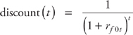
where discount(t) is the relevant discount factor, determining the amount of discount applied to items scheduled to arrive t periods from now. A discount factor equal to 1 means that future scheduled arrivals are undiscounted, relative to current arrivals. A discount factor less than 1 means future arrivals are discounted, which is usually the case. If, say, the discount factor equals 0.99 for goods arriving 1 period from now, they are worth less than current goods by an amount of 1 − 0.99 = 0.01 or 1 percent.

To determine appropriate discount factors, we can use posted prices in the market for riskless zero-coupon bonds. For a bond promising payment of $1,000 after t years, the face value is $1,000. The discount factor, discount(t), is then the ratio of the bond’s current price to its face value. Generally, the formula is

(3.4)

While the discount factor formula (3.4) is often handy enough, market outcomes for bonds are sometimes stated in terms of yields rather than prices. With rf0t being the yield to maturity on a zero-coupon risk-free bond issued at time 0 and maturing t periods in the future, we can restate our discount factor in terms of bond yields

(3.5)

Let us apply what we have learned so far to determine the economic harm caused by destruction of a stream of values in future years. Let yt be the value at time t of goods that were scheduled in that period, if not for economic harm. Using our formulas (3.2), (3.3), and (3.5), the harm associated with future losses is

(3.6)

For example, a factory’s accidental toxic spill may destroy a farmer’s ability to plant crops for 10 years, and the economic harm includes profits yt that would have been earned in each future year.

Business liability for economic harm is greater when the market discounts future earnings less, with lower bond yields rf0t. Conversely, liability is less when yields are higher. Over time, bond market conditions change and yields drift up and down, and these economic fluctuations affect business liability—particularly for economic harm that extends farther into the future.

Risk

We do not know exactly what will happen in the future, and economic harm is a business liability that is often not exactly known either.

Risk-Neutral Preferences

A simple way to handle uncertainty is to base projected future losses on expected values. Let E[yt] represent today’s expected value of an uncertain future value yt.10 The risk-neutral preference model, for pricing earnings streams, is

(3.7)

With risk-neutral preferences, uncertainty about the future affects price only through its effect on expected values E[yt]. This pricing model is appropriate if risk in the future earnings stream is considered unharmful, as is the case if such risk can be fully diversified by savvy investors.11

Liability is big if a business causes the loss of a superstar’s salary for a year, but it can also be big if an ordinary salary is lost for a long period of time. For example, when a business causes physical injury to someone, making them unable to continue working, the economic loss extends to the end of their expected working life. To evaluate the dollar amount of economic loss in such cases, one can use the pricing model (3.7) together with some assumptions of the expected amount of future earnings and the yields on short- and long-term riskless bonds.

Example 3.2 Pop Star Loss

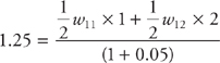
In an economy with a single future year of earnings (T = 1), let the interest rate be 5 percent, and suppose that an advertising company does economic harm to a client—a popular music performer—in terms of future earnings, with a future loss equal to $1 million with 50 percent chance, and $2 million with 50 percent chance. Suppose also that the earnings risk is fully diversifiable, and hence disregarded by financial markets. Applying the risk-neutral preference model (3.7), the current price of the lost future earnings is

Expected earnings are

E[y1] = prob(y1 = 1) × 1 + prob(y1 = 2) × 2

and since the probabilities prob(y1 = 1) and prob(y1 = 2) are each ½, E[y1] = 1.5. The riskless bond yield rf01 is just the interest rate, equal to 0.05, so the price of future earnings is

Business liability, due to economic harm, is then $1.43 million.

Example 3.3 Blue Collar Loss

A construction worker is injured on a job site by a cement truck with a faulty cement chute. The injury is disabling, preventing future work. The worker’s earnings would have been expected to grow by 3 percent each year, for the next 30 years. The yield on riskless bonds is 2 percent for future years 1 through 15 and 4 percent for future years 16 through 30. Applying formula (3.7), economic loss associated with future earnings is

(3.8)

The expression (3.8) involves the sum of 30 year-specific numbers. The calculation can be done using a pocket calculator, but a computer and high-precision mathematical software are more efficient and less prone to error. In this and all subsequent examples in this book, the author uses Stata software to set up calculations and create tables of results.

Table 3.1 shows the year-by-year expected earnings, for early years t = 1, 2, …, 5 and later years t = 26, 27, …, 30, with earnings in a given year equal to 30,000 × (1.03)t. It also shows the discount factor for each year, equal to 1/(1 + rf0t)t, by which expected earnings are reduced to expected loss in each year.12 The final column shows the cumulative loss in each year, equal to the losses in that year and all previous years. The final value in the cumulative column is the total loss, equal to $847,607.

Table 3.1 Economic loss, blue collar worker

Year	Expected earnings	Discount factor	Expected loss	Cumulative loss
1	30,900	0.98	30,294	30,294
2	31,827	0.961	30,591	60,885
3	32,782	0.942	30,891	91,776
4	33,765	0.924	31,194	122,970
5	34,778	0.906	31,500	154,470
...	...	...	...	...
26	64,698	0.361	23,336	756,486
27	66,639	0.347	23,111	779,597
28	68,638	0.333	22,889	802,487
29	70,697	0.321	22,669	825,156
30	72,818	0.308	22,451	847,607

Risk-Averse Preferences

Some value streams carry risk that could not be diversified away by investors who spread money across many earnings streams. Such risk is called undiversifiable, or systematic, risk. The risk-neutral preference model tends to overprice earnings streams that carry systematic risk. The presence of such risk makes the streams less attractive, and the model misses this. The model can be generalized to account for systematic risk, as follows

(3.9)

where wt, t = 1, 2, …, T are random weights, the same for all earnings streams. The weights wt take on positive number values, and like yt are uncertain, but their expected value is always the same and equal to 1.13 The pricing model (3.9) is general in the sense that it does not rely on risk-neutral preference toward risk. It is also more complicated, owing to the presence of expectations and the weight variable, but the extra effort is worthwhile when there is important uncertainty about future earnings.

To further interpret the general pricing model, for each future period t one can interpret the expected value E[wt yt] as the certainty equivalent of risky earnings yt—the amount of certain, or sure, earnings that a risk-averse investor would be willing to accept in trade for risky earnings. If yt is unrelated to systematic risk, then the certainty equivalent of yt coincides with its expected value E[yt]. If instead yt is related to systematic risk, then its certainty equivalent E[wt yt] may fall below E[yt] or exceed it, depending on whether the risk relationship is negative or positive.

The random weights wt in the pricing model (3.9) reflect investors’ attitudes toward risk. The relationship between wt and yt determines the impact of risk on the present value of earnings. For risky earnings in a future year t, if the certainty equivalent E[wt yt] equals expected earnings E[yt], then the weight variable wt and earnings variable yt are uncorrelated—having no linear statistical relationship with each other. On the other hand, if the certainty equivalent falls below expected earnings, then the weight and earnings variables are negatively correlated—having a negative linear relationship. If the certainty equivalent exceeds expected earnings, then the weight and earnings variables are positively correlated.

Example 3.4 Blue Chip Loss

Let the setup be the same as in Example 3.2, but suppose the advertiser’s economic harm is to a Blue Chip big business client rather than a pop music star, and that all earnings loss is systematic and undiversifiable. Investors fear systematic risk, and this causes the price of future earnings to be less than the risk-neutral value 1.43 found in Example 3.2 without such risk.

To price the risky earnings, consider what a reasonable person or institution would pay for the opportunity to collect next year either $1 million or $2 million, each with 50 percent chance. The riskless financial alternative pays 5 percent interest. Is $1.25 million a reasonable price for the risky earnings opportunity? It is cheaper than the $1.43 million risk-neutral price, by 13 percent. This risk discount is a substantial reduction in liability for the advertising company that caused the earnings loss. Whether it is cheap enough, to adjust for risk, depends on how much people fear financial risk—we will return to that point later on.

Right or wrong, the $1.25 million price for future risky earnings is consistent with the general pricing model (3.9). To show this, it is enough to find values for the random weight variable w1 such that a price of 1.25 on the left side of Equation 3.9 matches the value on the right side. Let s1 and s2 denote the two random outcomes, or “states of nature,” with future earnings of $1 million in the first state and $2 million in the second state. The random weight w1 takes on two possible values, the first in state 1 and the second in state 2, denoted by w11 and w12, respectively. Similarly, let y11 and y12 be the state-specific values of random future earnings y1. The general pricing model provides the formula

(3.10)

Plugging in values for price, probabilities, interest rate, and state-specific weight and earning values, formula (3.10) reduces to an equation in the weight values w11 and w12

(3.11)

There are infinitely many pairs of numbers (w11, w12) that satisfy condition (3.11), but not all fit the situation at hand. The weight’s expected value equals 1, by assumption, in which case

E[w1] = prob(s1)w11 + prob(s2)w12 = 1

The two state probabilities are each assumed to be equal to ½, and so the weight values must satisfy

(3.12)

The two weight restrictions (3.11) and (3.12) have a single common solution, this being

w₁₁ = 1.38, w₁₂ = 0.63 (3.13)

These weight values are positive, and otherwise fit the setup of the general pricing model.

Table 3.2 summarizes the inputs to the pricing exercise, with risky and riskless earnings in different states, and random weights. With this specification, the model implies a price of $1.25 million for random future earnings.

Table 3.2 Earnings and returns, risky and riskless

State	Probability	Riskless earnings	Risky earnings	Random weight	Riskless return	Risky return
1	0.5	1	1	1.38	0.05	−0.2
2	0.5	1	2	0.63	0.05	0.6

The output of the pricing formula (3.10) is a price for earnings streams. To understand this conversion of inputs to output, restate the formula in terms of the risky earning’s certainty equivalent

(3.14)

With the expression E[w1 y1] being the certainty equivalent of risky earnings y1

E[w₁y₁] = prob(s₁)w₁₁y₁₁ + prob(s₂)w₁₂y₁₂ (3.15)

Plugging in unknowns, earnings’ certainty equivalent is

which equals 1.344. By comparison, expected earnings are

a larger number: Earnings’ expected value exceeds its certainty equivalent. A seemingly different, but logically equivalent, statement is that the weight variable w1 and earnings variable y1 are negatively correlated. This negative correlation exists since the weight variable’s value is higher in state 1 than in state 2, while the opposite is true of the earnings variable—the weight and earnings variables move in opposite directions.

Business liability for the loss of future earnings is lowered by the presence of systematic risk, by an amount of $1.43 − 1.25 = $0.18 million. Risk causes earnings’ certainty equivalent to be less than its expected value, and this in turn lowers the price of future earnings. Risk also causes the weight variable wt to be negatively correlated with earnings, an equivalent condition that again lowers earnings price.

A lower price for future earnings makes them more attractive, all else equal. It also raises the return on investment, this being profit (earnings minus price) divided by price.

In Table 3.2, riskless earnings equal $1 million in each state of nature. The market price of the riskless opportunity is 0.95, so the return is (1 − 0.95)/0.95 = 1.05 in each state. On the other hand, risky earnings equal 1 in state 1 and 2 in state 2, and with price being 1.25, the investment return is (1 − 1.25)/1.25 = −0.2 in state 1 and (2 − 1.25)/1.25 = 0.6 in state 2.

Earnings opportunities are more attractive when their expected returns are higher. The expected return, also called mean return, is the probability-weighted sum of return values, analogous to expected earnings. Expected returns are higher when expected earnings are higher and when the earning stream’s price is lower.

For the Blue Chip case (Example 3.4), Table 3.3 shows mean earnings and returns for the riskless bond and risky business earnings. The mean return is higher for the risky opportunity than for the riskless one. The difference here between the risky and riskless returns is 0.2 − 0.05 = 0.15, or 15 percent, a risk premium for bearing risk. Compared to a broad portfolio of risky assets, a 15 percent risk premium is pretty high. Commonly cited risk premium values, for stock portfolios, are in the range of 5 to 10 percent.14 If in fact the Blue Chip company’s earnings are synonymous with systematic risk, then a 15 percent risk premium seems excessive, in which case the fair market price may not be $1.25 million but instead some higher number. For instance, if price is $1.35 million, then the risk premium is 0.061 or 6.1 percent. A higher price for earnings means greater harm in their loss, and more liability to the business that causes the loss.

Table 3.3 Mean and standard deviation, earnings, and returns

Variable	Mean	Standard deviation
Riskless earnings	1	0
Risky earnings	1.5	0.5
Riskless return	0.05	0
Risky return	0.2	0.4

A higher expected return on risky earnings, versus riskless ones, is compensation for risk. One measure of risk in earnings y is variance, this being the expected squared difference between earnings and their mean value

Variance measures the spread, or dispersion, in the values of the random variable y. A closely related measure of risk is standard deviation

Standard deviation takes variance as input and converts it into a number that has the same units as the variable y. Risky earnings have positive variance and riskless earnings have zero variance. The same principle holds for risky and riskless returns; they too have some variance Var[r] and standard deviation Std[r]. In Table 3.2, the risky return has positive variance which, once converted to standard deviation, equals 0.4, whereas the riskless return has standard deviation equal to 0.

The price of risky earnings must be low enough so that expected return sufficiently compensates for positive variance. A useful measure of the trade-off between risk and expected return is the Sharpe ratio—the ratio of expected excess return to the standard deviation of return, with excess return being the difference between the risky asset’s return and the riskless asset’s return. Its formula is

A higher Sharpe ratio indicates more compensation for risk-bearing. A lower price for risky earnings drives up both the mean and standard deviation of risky return and also drives up the Sharpe ratio. For a business causing the wrongful loss of earnings, a lower earnings price means less liability and a higher Sharpe ratio.

For the Blue Chip case (Example 3.4), the Sharpe ratio is

If instead price is $1.35 million, then the implied Sharpe ratio is lower, equal to 0.165. To put these numbers in historical perspective, for a broad market portfolio of U.S. stocks, the long-term historical average excess return is 7.74 percent while the historical sample standard deviation of returns is 64.91 percent,15 producing a Sharpe ratio of 7.74/64.91, or 0.12.

The contrast between the Pop Star and Blue Chip cases (Examples 3.2 and 3.4) illustrates the potential impact of systematic risk on business liability. Liability is greater in the Pop Star case because the star’s earnings bear no systematic risk, unlike the Blue Chip company’s. What if, instead, the pop star’s future earnings bear some systematic risk, due to the public’s concern about buying expensive concert tickets in trying economic times? Then the advertiser’s business liability for the pop star’s lost earnings should be somewhere between the risk-neutral value of $1.43 million and the value that compensates for purely systematic risk—$1.25 million (see Example 3.4). Percentage-wise, the amount of risk discount—off the risk-neutral value—should be somewhere between 0 and 13 percent. A risk discount of, say, 7 percent would make business liability equal to $1.33 million.

Earnings streams that bear systematic risk are priced at a discount relative to those that do not, a fact that we can express as follows:

(3.16)

With price(stream) being the stream’s price according to the general model (3.9), pricerisk-neutral(stream) being the price according to the risk-neutral model (3.7), and d being a risk discount factor. In the Blue Chip case (Example 3.4), d = 0.013 or 13 percent. Earnings that bear no systematic risk have no such discount and so d = 0, as in the Pop Star case.

The idea of a risk discount makes it relatively simple to evaluate business liability for loss of risky future earnings. To find the amount of liability, one can take two steps.

1. 1.Find the risk-neutral price of future earnings.
2. 2.Discount the risk-neutral price to adjust for risk and find economic loss.

The amount of risk discount, in the second step, depends on the extent to which lost earnings bear systematic risk. Determining the risk discount, and business liability for earnings loss, requires an understanding of the extent of risk and financial markets’ attitude toward it. A simple starting point is to assume that the risk is entirely systematic and coincides with the risk of a well-balanced portfolio of risky assets, in which case a reasonable risk discount can be gleaned from earnings’ expected return and variance. One can then adjust the risk discount, up or down, to reflect a more complex relationship between earnings and the general market for risk.

For future earnings in two or more future periods, the two-step liability calculation works, just as in the case of one future period. Finding a reasonable risk discount factor d again requires careful thought about the trade-off between risk and expected return. In principle, the relevant value of d may depend on the time horizon T, but such dependence disappears if one makes the following simplifying assumption

E[m_ry_r] = (1 – d)E[y_r] (3.17)

for some d and all t = 1, 2, …, T. An equivalent assumption is that the ratio of certainty equivalent to expected earnings is the same for all future periods t. The Appendix to this chapter discusses conditions under which this assumption holds.

Risk Hedges

Some earnings streams run counter to the overall economy. They counter systematic risk and act as a hedge—taking random values that offset the ups and downs of overall market value fluctuation. An example is the profit stream of a rum company, with the idea that people drink more hard alcohol during economic recessions than in economic expansions. A hedge earnings stream is priced higher than a stream that bears—rather than counters—systematic risk. For a hedge, the earnings stream’s price exceeds that of a stream that bears no relation to systematic risk. The pricing relationship (3.17) works for a hedge, but the risk discount factor d is a negative number.

Example 3.5 Rum Ruin

Two rum companies merge and, with their combined resources, are able to slash price and withstand losses while their remaining competitor is driven out of business. Their actions reduce economic competition and so cause economic harm. To describe this harm, suppose as in Example 3.3 that there are a single future period and two states of nature—states 1 and 2. In state 1, the ruined rum company would have earned $2 million next year, but for the wrongful act. In state 2, it would have earned $1 million. These earnings are counter to those of the general economy—which is stronger in state 1 than in state 2. Investors can use these earnings to hedge against systematic risk, and for this the rum company’s earnings would have been priced at premium. Assuming as earlier a 5 percent interest rate, the risk-neutral price is the same as for the Blue Chip company, equal to $1.43 million. Applying the general pricing formula (3.9) with the weight values w appearing in Table 3.2, the risk-adjusted price of the rum company’s future earnings is 1.61, this being the business liability of the newly merged companies. The risk-adjusted price is 13 percent above the risk-neutral price, and so the pricing relationship (3.16) applies with d = −0.13.

For a hedge, the certainty equivalent of future earnings exceeds expected earnings. Investors are willing to pay extra to get risky earnings rather than riskless ones, because the risk here offsets systematic risk elsewhere. Casting the certainty equivalent in terms of the weight variables wt introduced earlier, for a hedge the weight variable wt is positively correlated with earnings yt.16 For a business that causes the wrongful loss of someone’s earnings, if earnings are a hedge then they are priced higher than without the hedge, and business liability is greater.

To recap, if a business causes a wrongful loss of someone’s earnings stream, uncertainty in that stream can do one of three things to business liability: (a) it can decrease liability if the earnings stream carries systematic risk, (b) it can increase liability if the stream counters systematic risk, and (c) it can leave liability unchanged if the stream bears no relation to systematic risk.

Implicit Rate of Return

The present value of a future earnings stream depends on expected earnings, bond yields, and exposure to systematic risk. Present value is higher when expected earnings are higher, bond yields are lower, and systematic risk is either absent or offset by earnings variation. With multiple influences on present value, the pricing formulas (3.6), (3.7), and (3.9) are complex.

A relatively simple way to describe the impact of risk on the price of earnings stream is to find a discount rate (call it r*), for which the price of the stream matches the risk-neutral pricing model (3.7), assuming that all bond yields equal r*:

(3.18)

The discount rate r* is the implicit rate of return—the hypothetical discount rate at which the present value of expected earnings matches the earnings’ market price. Higher values of the riskless bond yields rf 0t, and more exposure to systematic risk, raise the implicit rate of return. Because the implicit rate of return generates a present value that matches market price, it is also called the required rate of return—the smallest rate of return that investors would accept to buy the earnings stream. If the earnings stream represents a claim to a company’s earnings, the implicit rate of return is also the company’s cost of capital—the expected rate of return that the market requires in order to attract funds to the company.

To illustrate the idea of implicit return, consider again the Blue Chip earnings loss (Example 3.4). The earnings stream has a price of $1.25 million and expected earnings of $1.5 million. The implicit rate of return r* solves the equation

(3.19)

in which case r* = 0.20, higher than the riskless bond yield rf 01 = 0.05 due to systematic risk. The Blue Chip implicit return is the same as the expected return.

For a business that causes a wrongful loss of future earnings to others, business liability is higher when earnings’ implicit or required return is lower, since then there is less discounting of earnings.

Options

Business liability includes the economic harm associated with earnings lost in the past and present, and those expected in the future. Liability extends to some situations where earnings could have been made, but for the business’s harm, regardless of the likelihood that they would be made. In other words, economic harm can arise by depriving people of the option to pursue economic opportunities, whether or not the option is actually chosen. So long as the option has market value, and hence can be exchanged for other opportunities, the holder of the option is made worse off by being deprived of it.

The options available to businesses, to pursue future earnings opportunities, are called real options, as they come up in the real day-to-day operation of business.17 By contrast, the options available to everyone for buying and selling publically traded stocks and commodities are called financial options. A wrongful loss of financial or real options is a business liability, but so too is the loss of any option to pursue economic opportunity in the future.

Determining the value of options is sometimes easy, and sometimes not. Prices for regularly traded stock and commodity options are posted each business day in the newspaper. Less frequently traded financial options present more of a valuation problem. For any economic option, with or without a posted market price, economic theory provides a pricing model via formula (3.9). To apply this model, one must first determine the underlying economic opportunity and the nature of the option to seize it. The underlying opportunity, bundled with the option details, begets a derived—or derivative—earnings opportunity.18

If the underlying opportunity is earnings y1 for future years t = 1, 2, …, T, then the derivative opportunity is also a sequence of future earnings; call them yt*. Applying formula (3.9) to yt* in place of yt provides the option’s value.19

Example 3.6 Land Developer

A construction company buys an option to develop a piece of land. The option guarantees the developer exclusive right to buy the land next year, for $10 million. If the company buys the land in year 1, it builds an office complex and sells it in year 2 for $15 million. At time 0, riskless bond yields are 1 percent for 1-year and 2-year maturities. A competing construction company learns of the option agreement and makes the land owner a better offer. The land owner breaches the original option contract, causing economic harm.19

The underlying economic opportunity is the $15 million of earnings available in year 2. To get that opportunity, the construction company pays $10 million in year 1 and also pays the option price in year 0. Underlying earnings are y2 = 15 million and derived earnings are y1* = −10 million and y2* = 15 million. The option value is the price of the earnings stream yt*, to which the general pricing formula (3.9) applies. Neither the underlying nor derived earnings are uncertain, so the pricing formula takes the simpler form (3.7). The option’s price is

(3.20)

Plugging in values for y1*, y2*, rf 01, and rf 02 into (3.20) yields

(3.21)

which equals 4.8. If the developer had paid $4.8 million for the option, then this dollar amount would also be the economic harm caused by the option’s loss. If the developer paid less, say $2 million, then economic harm would again be $4.8 million because the developer lost both the option’s purchase price (2 million) and the savings afforded by buying below the option’s approximate market price (4.8 million).

In Example 3.6, a business is wrongfully deprived of a real option. The mechanics of the option are similar to that of a customer’s layaway plan for buying a big-ticket item at a retail store: The customer pre-pays a portion of the purchase price, hence guaranteeing ultimate delivery. A modern variant of this is the warehouse shopping club—with an annual fee and discounted consumer prices, as is the issuance of “frequent customer” points by a business to loyal customers—with points redeemable as a discount off future purchases.

Example 3.7 Warehouse Club Bust

A consumer “warehouse club” company charges $50 per member, and each member gets a 20 percent discount off market prices for consumer items for a whole year. The club has 10,000 paying members, but is destroyed by a tornado, causing the company to breach its contract permanently, just after all members renewed for another year. The total loss to all customers is the savings that would have been afforded by the club in the coming year. Let x1 be the total amount customers would have spent, but for the contract breach. Given the loss of their 20 percent discount, they will now have to spend an extra

to get the same goods at regular prices. Supposing, for simplicity, that all spending would have been done at the end of the year, the price at time 0 of the savings opportunity is also the price of the customers’ option to buy at discount

Suppose that x1 is unrelated to systematic risk, in which case y1 is also. Let expected spending E[x1] be $50 million and let the interest rate be 1 percent. Then expected savings is E[y1] = ((1/.8) - 1)E[x1] = 12.5 and the option’s value is

(3.23)

The economic harm, caused by contract breach, is $12.38 million. This dollar amount is likely to exceed the funds collected as annual fees, since shoppers expect to recoup the fee and get additional savings by being club members. With a $50 fee and 10,000 members, the total fee is $500,000, much less than the economic harm.

If a shopper spending x1 carries systematic risk, then one can reapply pricing formula (3.22) but with a discount for risk. A risk discount of, say, 13 percent would reduce economic harm to $10.8 million.

The shopping club example is about an option available to consumers, but like the land developer example, it presupposes that the option—once purchased—will certainly be exercised. Once a club member, shoppers will buy club goods; once land is optioned, it will be developed. Any uncertainty comes from the underlying earnings.

Some options carry value even though there is a significant chance that they will not be exercised. A land developer that options a piece of land now may not yet have funds a year hence to build, and so may not seize the option to buy and build on the land. Furthermore, poor economic conditions may lower the developer’s expected earnings from the project, making the option’s exercise unprofitable.

Example 3.8 Land Developer, Revisited

Assume the situation in Example 3.6, but now suppose that the profitability of land development changes over time. With a land option purchased at time 0, subsequent events at time 1 affect the profitability of developing the land and selling the finished project at time 2. At time 1, one of two states of nature occur, either state s1 or s2. At time 0, denote the probabilities of these states’ occurrences as prob(s1) and prob(s2), respectively. If at time 1 state s1 happens, then the developer’s expected period-2 earning from the project is E1[y2] = $25 million. If instead s2 happens, then E1[y2] = $10 million.

At time 1, the developer will seize the option to buy and build only if the economic opportunity generates positive value. If period-2 earnings are unrelated to systematic risk, then the period-1 value generated by the buy-and-build choice is

(3.24)

with derived earnings y1* equal to −1 times the land’s purchase price and y2* equal to period-2 project earnings, and with rf12 being the yield in year 1 for a bond maturing in year 2. The developer exercises the build option in year 1 if price1(y1*, y2*) is positive. Stepping back to year 0, the choice to build is uncertain since E1[y2*] is unknown at that time. Another possible unknown is the next-period bond yield rf12, but for simplicity suppose this is known to be 1 percent. Plugging in inputs to (3.24), in state s1 the build choice has time-1 value

(3.25)

While in state s2 it has value

(3.26)

The developer will buy and build in the first state, as value is positive, but not in the second.

At time 0, expected derived earnings in year 1 are the probability-weighted sum of possible values

(3.27)

Which simplifies to

(3.28)

Expected derived earnings in year 2 are

(3.29)

At time 0, the option’s value is

(3.30)

Let the probabilities prob(s1) and prob(s2) each equal 50 percent. Applying formulas (3.28) and (3.29), expected derived earnings are E[y1*] = −5 and E[y2*] = 12.5. With bond yields each equal to 1 percent, formula (3.30) provides the option price

(3.31)

which equals 7.30. In this revised version of the building developer example, economic harm associated with the option’s loss is now $7.3 million.

Financial options, on stocks and other assets, carry uncertainty about the underlying asset’s value and also about the future choice to exercise (or not) the option. The future exercise choice itself may depend on future market conditions, but ultimately options are just another type of earnings stream, and so can be priced using the general formula (3.9). The task can be simplified if one makes stronger assumptions about the underlying economic opportunities. Popular models, which incorporate such assumptions, include the binomial option pricing model for stocks and other financial assets, which assumes two uncertain states of the world in each future period, similar to Example 3.6. Similar to the binomial model is the Black–Scholes model, which assumes that economic opportunity unfolds over a continuum of dates t rather than over a discrete set of years or months and so on, but gives near-identical results when the period length is short.

Use of binomial and Black–Scholes option pricing models simplifies option valuation, provided that models’ assumptions are appropriate. Business liability, for the wrongful loss of an option, is more easily determined in such cases. In general, the all-purpose pricing model (3.9) of earnings streams is available to price options and all other earnings streams, but the end result sometimes requires considerable thought, analysis, and computer work.20

APPENDIX

Chapter 3 explored economic loss manifest as a loss of some earnings stream or a sequence of scheduled payments. It also explored losses manifest as options. A fundamental formula, for pricing an earnings stream, is the law of one price which, in Chapter 3, is stated as formula (3.9). This formula is based on simplifying assumptions, essentially that markets are efficient and well-working, but otherwise applies to many situations. Because it is a general formula, (3.9) takes some work in getting it focused to any particular application. In Chapter 3, follow-up formulas (3.17) and (3.18) are attempts to bring (3.9) to bear in more practical terms. But to get these follow-up formulas to work, some additional motivation or explanation is needed at some point. The technical material in all these formulas may breach the boundaries of some readers’ math comfort zone, and a more in-depth discussion of them is likely to stray further in that direction. For this reason, the in-depth discussion appears here in the Appendix to Chapter 3, as a resource to those readers who want it.

Risk-Averse Asset Pricing

The law of one price, manifest as formula (3.9) in the text, is a standard asset pricing formula from financial economics. It accommodates the fact that the typical individual facing a stream of risky future earnings is likely to be averse to risk. The formula gives a price for risky earnings streams, with discounts for earnings risk. If one risky activity has higher earnings risk than another, the discount for risk will be higher for the more risky activity, ceteris paribus. Similarly, if some activity has higher than average risk, then it may have a higher than average discount for risk. On the other hand, if people can diversify away a given earnings stream’s risk by holding many investments in a portfolio, then they may not be worried about the risk. With diversification, only undiversifiable or systematic risk is priced in the marketplace.

Assuming that people dislike financial risk, earnings streams are worth less if they carry systematic risk than if they do not. In the general pricing model (3.9), the price effect of systematic risk is reflected in the expected products E[wtyt]. Without systematic risk, these products are the same as expected earnings E[yt], but with such risk they are less

(3A.1)

Since the random weight wt itself equals 1 on average, the inequality (3A.1) can happen only if the value of wt tends to move in the opposite direction as that of yt ; in other words, if there is negative correlation between wt and yt . This negative correlation lowers the price of earnings stream. One can make this fact more explicit by rewriting the pricing model in terms of correlation21

(3A.2)

where Corr[wt,yt] is the correlation, Std[wt] is the standard deviation of wt, and Std[yt] is the standard deviation of yt . With systematic risk in the earnings stream the random future values wt and yt are negatively correlated, and so Corr[wt,yt] < 0, whereas with no such risk there is no correlation, and so Corr[wt,yt] = 0 and pricing coincides with the risk-neutral model (3.7) in the text.

To carry out risk-adjusted pricing of earnings streams, one needs more information about the random weights wt that appear in either formula (3.9) or its restatement (3A.2). The weights reflect society’s aversion to risk, and so carry with them some economic theory about risk aversion. The general theory of risk aversion is beyond the scope of this book, but a simple form of this theory identifies the weights wt in terms of market return—the investment return on a fully diversified portfolio of assets. Denoting by Rm0t the gross multiperiod return on the market portfolio between dates 0 and t, under simplifying assumptions the weights wt are determined by Rm0t as follows

(3A.3)

for some positive constant b. If one can observe market returns Rm0t and determine their expected values, then one can find the weights wt and the prices of earnings streams. There remains the problem of getting a value for the constant b, but for this economic theory again proves useful. Denoting by Rmt the gross 1-period return on the market portfolio between dates t − 1 and t, and by Rft the gross 1-period riskless return on a bond, the theoretical value of b is

(3A.4)

where “ln” denotes natural logarithm and “Var” denotes variance. The value of b is at least ½ because, according to the theory, the single-period expected (log) return exceeds the (log).

Applying these ideas from financial economics, consider the market value of a firm’s owners’ equity in the firm. In theory, this value should equate to the price of the firm’s expected risk-adjusted future income stream.

Example 3A.1 Closely held corporation, not publically traded. Current projections are that the company’s future earnings yt are expected to be $1 million per year, with standard deviation $100,000 and a correlation 0.20 (20 percent) with the asset pricing kernel mt, which itself has standard deviation 0.05. Consider the present value of the company’s earnings opportunities through year T = 20, assuming that bond yields rt are 0.02 (2 percent) for each future year t = 1, 2…, 20. Applying formula (3A.3), the expected product E[mtyt] is

E[mtyt] = (0.052) × (100,000)2(0.20)2 + 1,000,000 = 1,010,000

We then apply (A1.2) to compute the present value of future earnings as

1In Chapter 4, we will turn to the question of whether or not a business is liable at all.

2Alternatively, the court might choose a value for economic compensation that achieves the lowest cost to society, but if such costs ultimately rely on utility arguments, then the result should be the same as when the court tries to maximize social utility or welfare U(C).

3This is one interpretation of the “make-whole” principle in tort law; see the following discussion.

4While common sense, it may be that an injured party’s utility cannot be restored to its pre-injury level, as when a commercial truck causes catastrophic and permanent injury to another driver on the road.

5Even if the specific economic opportunity is not available for sale in the marketplace, there may be a close substitute available.

6In stark contrast to this idyllic rational economic interpretation of the court’s approach to liability and economic damages is the “reptile theory of trial strategy” in which the plaintiff ’s lawyers may try to appeal to the reptilian part of jurors’ brains and shock them into focusing on public safety rather than economic losses in a particular case. While a popular tactic, defense lawyers are now used to dealing with it. On the whole, the idea of a rational and economics-oriented court remains a central theme in the law and economics school of thought, and is a fruitful perspective on cases of business liability.

7In Chapter 3, we will discuss evidence and proof of economic harm.

8In the literature on asset pricing, this formula is sometimes called the law of one price. Different statements of this fundamental result include equation (22.2) of Principles of Financial Economics (by Leroy and Werner 2001, p. 228), equation (5.14) of Asset Pricing Theory (by Skiadas 2009, p. 150), and the equation of Asset Pricing (by Cochrane 2001, p. 26).

9On the right-hand side of this formula is the number (3.1) that labels it. I will sometimes refer to formulas by their labels, when applying them later on.

10With yt being a random variable and unknown today, the expected value E[ yt ] is nonrandom and known today. In the language of probability and statistics, E[ yt ] is the mean value of random variable yt. If yt can take only one of finitely many possible values, then E[ yt ] is the probability-weighted average of those values.

11Another interpretation of risk-neutral asset pricing is that the relevant market participants have perfect foresight about future market conditions, resulting in perfect foresight equilibrium. For discussion, see “The Value of Future Earnings in Perfect Foresight Equilibrium” (Journal of Forensic Economics 21, No. 1, 2011) by the author (Scott Gilbert).

12That is, “expected loss” in Table 3.1 equals “expected earnings” times “discount factor.”

13That is, E[wt ] = 1. The reason for this restriction is that for riskless earnings streams the expected product E[wt yt ] equals the product E[wt ]E[yt ] of expected values, and since the risk-neutral model (3.7) then holds, a match of equations (3.7) and (3.9) requires E[wt ] = 1.

14The historical average excess return on a broad portfolio of U.S. stocks is 7.74 percent, for the period July 1926 to November 2013, based on market excess return data provided online by Kenneth French, and the author’s calculation.

15The annualized historical average excess return on a broad portfolio of U.S. stocks is 7.74 percent, for the period July 1926 to November 2013, based on market excess return data provided online by Kenneth R. French at Dartmouth University, and the author’s calculation. The historical standard deviation (of monthly returns, annualized) is 64.91 percent over this same period.

16Since a hedge is supposed to generate earnings that move in the opposite direction of the general market, it may seem puzzling that they also move in the same direction as the weight variable wt. In the Appendix to this chapter, this puzzle is explained by casting wt as the inverse—so to speak—of general market conditions.

17Examples of real options include the right to deliver products to Canada and the right to exclusive production afforded by a patent.

18If it did not, the option would be worthless.

19The economic harm is not the transfer of opportunity from the first developer to the second. Indeed, the second developer may be better able to add economic value to the land. The harm is the damage to contracts generally, owing to breach of a given contract, weakening contracts and their ability to facilitate economic opportunity.

20The mathematics of the binomial and Black–Scholes option pricing models is advanced and beyond the intended scope of this book. For a segue between the asset pricing models discussed in this book and the mathematics of multiperiod option pricing models, see the article “The Valuation of Uncertain Income Streams and the Pricing of Options” (The Bell Economics Journal 7, No. 2, 1976) by Mark Rubenstein.

21For this we apply the assumption E[wt] = 1 to get E[wtyt] = E[yt] + Corr[wt,yt]Std[wt]Std[yt].