
Chapter 17
Discriminant Analysis and Logistic Regression Analysis
Learning Objectives
Upon completion of this chapter, you will be able to:
- Understand the concept and application of discriminant analysis and multiple discriminant analysis
- Interpret the discriminant analysis output obtained from statistical software
- Use Minitab and SPSS to perform discriminant analysis
- Understand the concept and application of logistic regression analysis
- Interpret the logistic regression analysis output obtained from the statistical software
- Use SPSS to perform logistic regression analysis
Research In Action: Camlin Ltd
The Indian stationery market can be categorized into school stationery, office stationery, paper products, and computer stationery. Increased spending on the educational sector by the government, improvement in educational standards and introduction of new categories of specialized education, and concentration on overall development of students have led to the speedy growth of the stationery market in India. The office-supplies segment is also growing rapidly. Opening of new commercial offices having multi-locational presence has helped organized players with scalability to serve across locations and offer diverse range of products. These factors have not only contributed to increased demand but also shifted sales from unorganized to organized sector with premium-quality products.1
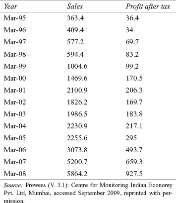
Mr D. P. Dandekar started Camlin in 1931. Camlin has come a long way from a company manufacturing ink powder in 1931 to a company manufacturing more than 2000 products, operating in various diverse fields. With more than 50,000 strong retailer network, prestigious foreign collaborations, large customer base, regular interaction with consumers by the sales force, and participation in international trade fairs, such as Paperworld in Frankfurt, it has now become a trusted household name all over India. It first launched the hobby range of colours in India. It has also introduced colour categories such as fine art colours, hobby colours, and fashion colours in India.2 Table 17.1 gives the income and profit after tax (in million rupees) of Camlin Ltd from 1994–1995 to 2008–2009.
TABLE 17.1 Income and profit after tax (in million rupees) of Camlin Ltd from 1994–1995 to 2008–2009
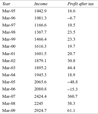
Source: Prowess (V. 3.1): Centre for Monitoring Indian Economy Pvt. Ltd, Mumbai, accessed September 2009, reprinted with permission.
Camlin, through its wholly owned arm Camlin Alfakids, plans to set up 200 preschools throughout the country within the next 5 years. Mr Nitin Pitale, President-Projects (New Business Development), told Business Line, “We have been looking to diversify into a new line of business for some time now. As we have strong brand equity among parents and children for our stationery and art products, we decided to get into the business of setting up and managing play schools.” The company is in the process of deciding whether these preschools will be company owned or franchised. Each proposed preschool will have an area over 8000 ft2 with facilities such as gardens, swimming pools, sandpits, and so on.3
Suppose Camlin Ltd wants to assess parent’s preference for the new playschool compared with two other established playschools and researchers have collected data on a categorical dependent variable (preference for three playschools including Camlin’s playschool). The independent variables have also been identified and data are collected on an interval scale. How will the researcher analyse the data? We have already discussed in the previous chapter that for applying multiple regression technique both the dependent and the independent variables should be interval scaled. In this case, the dependent variable is not interval scaled; hence, we are supposed to find another way of analysing the data. Discriminant analysis is a statistical technique to analyse the data when the dependent variable is categorical scaled and the independent variable is interval scaled. This chapter deals with the concept and application of discriminant analysis and another technique referred to as logistic regression analysis.
17.1 Discriminant Analysis
Chapter 17 specifically focuses on discriminant analysis and logistic (or logit) regression analysis. Use of these two multivariate techniques in business research is increasing day by day. Let us start the discussion by taking discriminant analysis first.
17.1.1 Introduction
We have already discussed that multiple regression analysis is used when both the dependent and independent variables are interval scaled. In real-life situations, there may be cases where the independent variables are interval scaled but the dependent variable is categorical scaled. Discriminant analysis is a technique of analysing data of this nature. For example, the dependent variable may be choice of a brand of refrigerator (Brand 1, Brand 2, and Brand 3) and the independent variables are ratings of attributes of the refrigerator on a 5-point Likert rating scale. As another example, a marketing research analyst may be interested in classifying a group of consumers into ‘satisfied with the product’ or ‘not satisfied with the product’ on the basis of few characteristics such as age, income, education, or any other characteristics that can be measured on a rating scale. Apart from the multiple regression technique, another technique that is becoming familiar and useful, especially in marketing applications, is the use of discriminant analysis in which an attempt is made to separate the observations into groups or clusters that have discriminating characteristics.1
Discriminant analysis is a technique of analysing data when the dependent variable is categorical and the independent variables are interval in nature.
17.1.2 Objectives of Discriminant Analysis
The following are the major objectives of discriminant analysis:
- Developing a discriminant function or determining a linear combination of independent variables to separate groups (of dependent variable) by maximizing between-group variance relative to within-group variance.
- Examining significant difference among the groups in light of the independent variables.
- Developing procedures for assigning new entrants whose characteristics are known but group identity is not known to one of the groups.
- Determining independent variables that contribute to most of the difference among the groups (of dependent variable).
Similar to multiple regression analysis, discriminant analysis also explores the relationship between the independent and the dependent variables. The difference between multiple regression and discriminant analyses can be examined in the light of the nature of the dependent variable that is categorical, when compared with metric, as in the case of multiple regression analysis. The independent variables are metric in both the cases of multiple regression and discriminant analyses. Thus, the dependent variable in discriminant analysis is categorical, and there are as many prescribed subgroups as there are categories.2
The difference between multiple regression and discriminant analyses can be examined in the light of the nature of the dependent variable that is categorical, when compared with metric, as in the case of multiple regression analysis. The independent variables are metric in both the cases of multiple regression and discriminant analyses.
17.1.3 Discriminant Analysis Model
Discriminant analysis model derives a linear combination of independent variables that discriminates best between groups on the value of a discriminant function. Discriminant analysis model can be presented in the following form:
Discriminant analysis model derives a linear combination of independent variables that discriminates best between groups on the value of a discriminant function.
![]()
where D is the discriminant score; b0, b1, b2,… bn are the discriminant coefficients; and x1, x2, x3,… xn are independent variables. The discriminant coefficients b0, b1, b2,… bn are estimated in such a way that the difference among the groups (of dependent variable) will be as high as possible by maximizing the between-group variance relative to the within-group variance.
17.1.4 Some Statistics Associated with Discriminant Analysis
Several statistical terms associated with discriminant analysis are described as follows:
Canonical correlation: It measures the degree of association between the discriminant scores and the groups (levels of dependent variable).
Centroids: The average (mean) value of the discriminant Score D for a particular category or group is referred as centroids. There will be one centroid for each group. For a two-group discriminant analysis, there will be two centroids, and for a three-group discriminant analysis, there will be three centroids. The averages for a group of all the functions are the group centroids.
Classification matrix: It gives a list of correctly classified and misclassified cases. The diagonal of the matrix exhibits correctly classified cases.
Unstandardized discriminant coefficients: These are multipliers of the independent variables in the discriminant function.
Discriminant function: Discriminant analysis generated linear combination of independent variables that best discriminate between the categories of dependent variable.
Discriminant scores: These can be computed by multiplying unstandardized discriminant coefficients by values of the independent variables and a constant term of the discriminant function is added to their sum.
Eigenvalue: For each discriminant function, Eigenvalues are computed by dividing between-group sum of squares by within-group sum of squares. A large eigenvalue implies a strong function.
F values and its significance: F values are same as it is computed in one-way analysis of variance (ANOVA). Its significance is tested by corresponding p values, which is the likelihood that the observed F value could occur by chance.
Pooled within-group correlation matrix: This is constructed by averaging the correlation matrices for all the groups.
Structure correlation: It is also known as discriminant loading and is the correlation between the independent variables and the discriminant function.
Wilks’ lambda (λ): For each predictor variable, the ratio of within-group to total-group sum of squares is called Wilks’ lambda. This is the proportion of total variance in the discriminant scores not explained by differences among groups. The value of Wilks’ lambda varies between 0 and 1. The value of lambda equal to 1 indicates that the group means are equal. This means that all the variance is explained by the factors other than the difference between these means. A small value of lambda indicates that the group means are apparently different.
Chi-square (χ2): It measures whether the two levels of the function significantly differ from each other based on the discriminant function. A high value of χ2 indicates that the functions significantly differ from each other.
17.1.5 Steps in Conducting Discriminant Analysis
Two-group discriminant analysis is conducted through a five-step procedure as follows: formulating problem, computing discriminant function coefficients, testing the statistical significance of the discriminant function, interpreting results generally obtained through statistical software, and concluding comments by performing classification and validating discriminant analysis. Figure 17.1 shows the five-step procedure of conducting discriminant analysis.
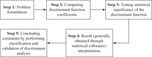
Figure 17.1 Five steps in conducting discriminant analysis
17.1.5.1 Formulating a Problem
Discriminant analysis starts with problem formulation by identifying the objective, the dependent variable, and the independent variables. The main feature of discriminant analysis is that the dependent variable must consist of two or more mutually exclusive and collectively exhaustive groups (categories). If the dependent variable is an interval or a ratio, it must first be categorised. For example, the dependent variable may be consumer satisfaction and is measured on a 5-point rating scale (strongly disagree to strongly agree with either agree or disagree in the middle). This can be further divided into three categories: dissatisfied (1, 2); neutral (3); and satisfied (4, 5).
As a next step, the sample is divided into two parts. First part of the sample is referred as estimation or analysis sample and is used for the estimation of the discriminant function. Second part of the sample is referred as hold-out or validation sample and is used for validating the discriminant function. To avoid data specific conclusions, validation of the discriminant function is important. The number of subjects (cases) in analysis and hold-out samples should be in proportion with the total sample. For example, if in the total sample 50% of the consumers are in the “satisfied” category and 50% of the consumers are in the “dissatisfied” category then the analysis and hold-out samples should also contain 50% consumers in the satisfied category and 50% in the dissatisfied category.
First part of the sample is referred as estimation or analysis sample and is used for the estimation of the discriminant function. Second part of the sample is referred as hold-out or validation sample and is used for the validation of the discriminant function.
The procedure of conducting discriminant analysis can be better explained by Example 17.1. In this example, four independent variables, such as age of the consumers, income of the consumers, attitude of the consumers towards shopping (measured on a 7-point rating scale), and occupation have been identified. The dependent variable is categorical and has two categories (groups): “satisfied” and “not satisfied.” Hence, this is a case of two-group discriminant analysis.
Example 17.1
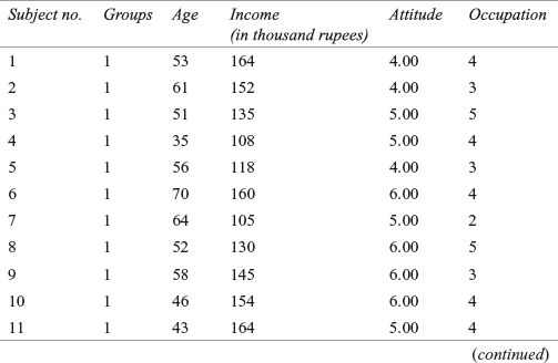
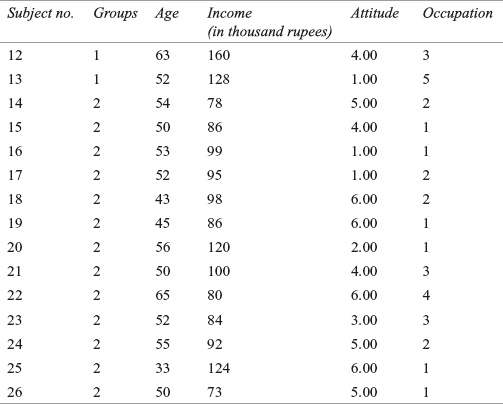
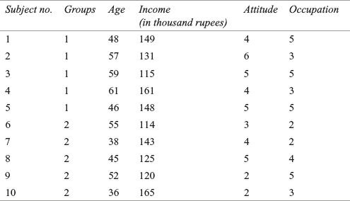
A garment company has launched a new brand of shirt. The company wants to categorize consumers into two groups—satisfied and not satisfied—related to some characteristics of the consumers during the last 2 years. The company conducted a survey and data were obtained from 36 consumers on the age of the consumers, income of the consumers, attitude of the consumers towards shopping (measured on a 7-point rating scale), and occupation. The data are given in Tables 17.2 (analysis sample) and 17.3 (hold-out sample).
TABLE 17.2 Data obtained for the garment company (analysis sample)
Solution SPSS generated output for Example 17.1 is shown in Figure 17.2.
17.1.5.2 Computing Discriminant Function Coefficient
After identifying the analysis sample, discriminant function coefficients are estimated. There are two methods to determine the discriminant function coefficients: direct method and stepwise method. This process is similar to the process of least square adopted for multiple regression. In the direct method, all the independent variables are included simultaneously, regardless of their discriminant power to estimate the discriminant function. In the stepwise method, the independent variables are entered sequentially based on their capacity to discriminate among groups.
There are two methods to determine the discriminant function coefficients: direct method and stepwise method.
As discussed earlier, there are four independent variables in Example 17.1, and each respondent’s individual discriminant score can be obtained by substituting his or her values for each of the four variables in the discriminant equation as below.
![]()
17.1.5.3 Testing Statistical Significance of the Discriminant Function
It is important to verify the significant level of the discriminant function. Null hypothesis can be statistically tested. Here, null hypothesis is framed as in the population; means of all discriminant functions in all the groups are equal. As discussed earlier, Wilks’ lambda (λ) is used for this purpose, which is the ratio of within-group sum of squares to the total group sum of squares. The Wilks’ lambda is a statistic that assesses whether the discriminant analysis is statistically significant.3 To test the significance of each independent variable, the corresponding F value is used. To test the significance of the discriminant function, chi-square transformation of Wilks’ λ is used. A high value of χ2 indicates that the functions significantly differ from each other. In Example 17.1, χ2 value is found to be 31.487 with the corresponding p value as 0. This value is significant at 99% confidence level. Hence, it can be concluded that the population means of all the discriminant functions in all the groups are not equal (acceptance of alternative hypothesis). It indicates that the discriminant function is statistically significant and further interpretation of the function can be proceeded.
To test the significance of each independent variable, the corresponding F value is used. To test the significance of the discriminant function, chi-square transformation of Wilks’ λ is used. A high value of χ2 indicates that the functions significantly differ from each other.
- 17.1.5.4 Result (Generally Obtained through Statistical Software) Interpretation
Figure 17.2(a) shows analysis case processing summary table. This is the first part of the discriminant analysis output. This gives a summary of the number of cases (weighted and unweighted) for each level (category) of the dependent variable and the values for each level.
Figure 17.2(b) shows group statistics, which gives the means and standard deviations for both the groups. From this figure, few preliminary observations about the groups can be made, and it clearly shows that the two groups are widely separated with respect to two variables: income and occupation. With respect to age, the difference between the two groups is minimal. A visible difference can also be observed in terms of the standard deviation of the two groups.
Figure 17.2(c) shows test of equity of group means. F statistic determines the variable that should be included in the model 4 and describes that when predictors (independent variables) are considered individually, only income and occupation significantly differ between the two groups. The last column of Table 17.2(c) is the p value corresponding to the F value and confirms that only income and occupation differ significantly between the two groups.
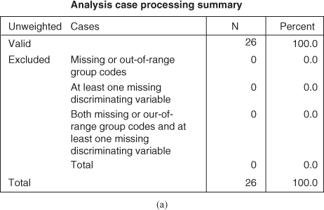
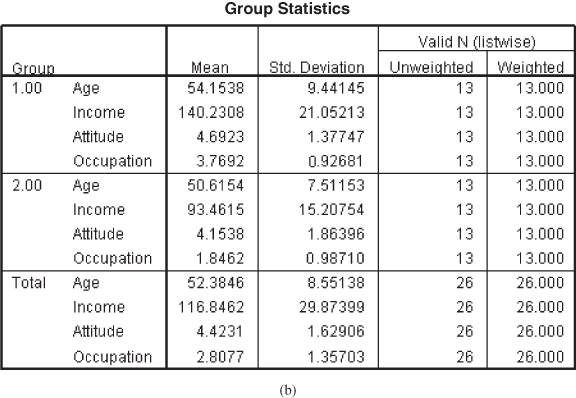
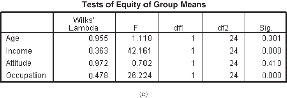
Figure 17.2 (a) Analysis case processing summary table, (b) Group statistics table, (c) Test of equity of group means table
Figure 17.2(d) shows pooled within-group matrices and indicates the degree of correlation between the predictors. From the figure, it can be observed clearly that there exist weak correlations (0 is no correlation) between the predictors. Thus, multi-collinearity will not be a problem.
Figure 17.2(e) shows Eigenvalues table, a large eigenvalue is an indication of a strong function. In Example 17.1, only one function is created with two levels of dependent variables. If there are three levels of dependent variables (a case of multiple discriminant analysis), 3 − 1 = 2 functions will be created. A maximum of n − 1 discriminant functions are mathematically possible when there are n groups.5 The function always accounts for 100% of the variance. As discussed earlier, canonical correlation measures the degree of association between the discriminant scores and the groups (levels of dependent variable). A high value of the canonical correlation indicates that a function discriminates well between the groups. Canonical correlation associated with the function is 0.872. Square of this value is given as (0.872)2 = 0.7603. This indicates that 76.03% of variance in the dependent variable can be attributed to this model.
Figure 17.2(f) shows Wilks’ lambda table. This is already described in the significance of the discriminant function determination Section (17.1.5.3).
Figure 17.2(g) shows standardized canonical discriminant function coefficients. From the figure, it can be noted that income is the most important predictor in discriminating between the groups followed by occupation, age, and attitude towards shopping, and note that F values associated with income and occupation are significant (see Figure 17.2(c)).
Figure 17.2(h) shows structure matrix table. The following line appears in the output of SPSS, “Pooled within-group correlations between discriminating variables and standardized canonical discriminant function variable ordered by absolute size of correlation within function.” Pooled values are the average of the group correlations. These structured correlations are referred as canonical loadings or discriminant loadings. The importance of a predictor variable can be judged by the magnitude of correlations. Higher the value of correlations, higher is the importance of the corresponding predictor.
Pooled values are the average of the group correlations. These structured correlations are referred as canonical loadings or discriminant loadings.
Figure 17.2(i) shows canonical discriminant function coefficients table, which gives an unstandardized coefficient and a constant value for the discriminant equation. As discussed earlier, after substituting the unstandardized coefficient values with the corresponding predictor and constant values, the discriminant equation can be written as
![]()
Figure 17.2(j) shows function at group centroids table. These are unstandardized canonical discriminant functions evaluated at group means and are obtained by placing the variable means for each group in the discriminant equation rather than placing the individual variable values. For the first group—satisfied—the group centroid is a positive value (1.714), and for the second group, it is an equal negative value (−1.714). The two scores are equal in absolute value but have opposite signs. From the discriminant equation, it can be noted that all the coefficients associated with the predictors have a positive sign. These results show that higher age, higher income, higher attitude towards shopping, and higher level of occupation are likely to result in satisfied consumers. Of the four predictors, only two have got a significant p value. Hence, it will be useful to develop a profile with these two statistically significant predictors.
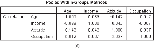
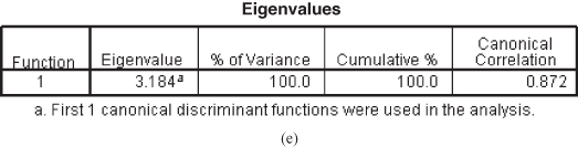
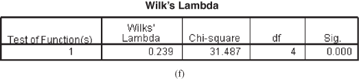
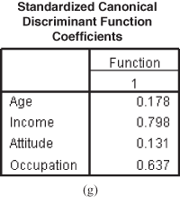
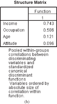
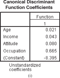
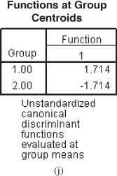
Figure 17.2 (d) Pooled within-group matrices table, (e) Eigenvalues table, (f) Wilks’ lambda table, (g) Standardized canonical discriminant function coefficients, (h) Structure matrix table, (i) Canonical discriminant function coefficients table, (j) Function at group centroids table
Figure 17.2(k) shows classification processing summary table.
Figure 17.2(l) shows prior probability for groups table. In the second column, the value 0.5 indicates that the groups are weighted equally.
- 17.1.5.5 Concluding Comments by Performing Classification and Validation of Discriminant Analysis
Figure 17.2(m) shows classification results table, which is a simple table of the number and percentage of subjects classified correctly and incorrectly. Both SPSS and Minitab offer cross-validation option. In leave-one-out-classification (Figure 17.7), the discriminant model is re-estimated as many times as the number of subjects in the sample. Each model leaves one subject and is used to predict that respondent. In other words, each subject in the analysis is classified from the function derived from all cases except itself. This is referred as U method.
Classification results table is a simple table of the number and percentage of subjects classified correctly and incorrectly.
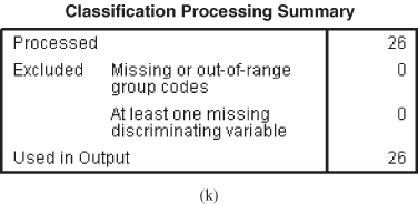
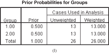
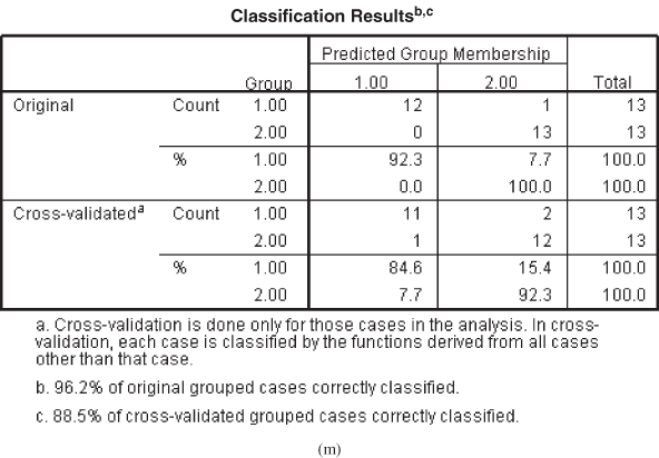
Figure 17.2 (k) Classification processing summary table, (l) Prior probabilities for groups table, (m) Classification results table
In the classification matrix, the diagonal elements of the matrix represent correct classification. The hit ratio, which is the percentage of cases correctly classified, can be obtained by summing the diagonal elements and dividing it by the total number of subjects. From Figure 17.2(m), it can be noted that the sum of the diagonal elements is 25 (i.e., 12 + 13 = 25), hence the hit ratio can be computed as 25/26 = 0.9615, and a line can be seen as a part of the SPSS output that “96.2% of the original grouped cases correctly classified.” This 96.2% is the hit ratio. One has to determine a good hit ratio. When the groups are equal in size (as in our case), the percentage of chance classification is one divided by the number of groups. Thus, in Example 17.1, the percentage of chance classification is 0.5 (i.e., 1/2 = 0.5). As a thumb rule, if the classification accuracy obtained from the discriminant analysis is 25% greater than that obtained from chance then the validity of the discriminant analysis is judged as satisfactory.
In the classification matrix, the diagonal elements of the matrix represent correct classification. The hit ratio, which is the percentage of cases correctly classified, can be obtained by summing the diagonal elements and dividing it by the total number of subjects.
As discussed, in the classification matrix, the numbers of cases correctly classified are 96.2%. One can argue that this figure is inflated, as the data for estimation are also used for validation. Leave-one-out-classification (cross-validation) correctly classifies 88.5% of the cases. The classification matrix of the hold-out sample (Figure 17.3) indicates that 100% of the cases are correctly classified and cross-validation indicates that 80% of the cases are correctly classified. Improvement over chance is more than 25%; hence, validity of the discriminant analysis is judged as satisfactory (no clear guideline is available for this, but few authors have suggested that the classification accuracy obtained from the discriminant analysis should be 25% more than the classification accuracy obtained by chance).
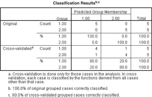
Figure 17.3 SPSS classification results table for hold-out sample
When the two groups considered in the discriminant analysis are of unequal size, then two criteria—the maximum chance criterion and the proportional chance criterion—can be used to judge the validity of the discriminant analysis. In the maximum chance criterion, a randomly selected subject should be assigned to a larger group to maximize the proportion of cases correctly classified. The proportional chance criterion allows the assignment of randomly selected subjects to a group on the basis of the original proportion in the sample. The formula used for this purpose is as follows: (proportion of individuals in Group 1)2 + (1 − proportion of individuals in Group 2)2.
In the maximum chance criterion, a randomly selected subject should be assigned to a larger group to maximize the proportion of cases correctly classified. The proportional chance criterion allows the assignment of randomly selected subjects to a group on the basis of the original proportion in the sample.
For example, a sample of size 100 is divided into two groups with 70 and 30 subjects in Groups 1 and 2, respectively. In this case, the proportional chance criterion will be equal to (0.70)2 + (0.30)2 = 0.58. Thus, a classification accuracy of 80% seems to have a good improvement over chance.
17.1.6 Using SPSS for Discriminant Analysis
In the case of using SPSS for discriminant analysis, click on Analyze/Classify/Discriminant. The Discriminant Analysis dialog box will appear on the screen (Figure 17.4). Enter the independent variables in the ‘Independents’ box and groups in the ‘Grouping Variable’ box and click on Define Range box (Figure 17.4). Discriminant Analysis: Define Range dialog box will appear on the screen (Figure 17.5). Enter 1 in the ‘Minimum’ box (first category of the group) and 2 in the ‘Maximum’ box (second category of the group) and click on Continue. The Discriminant Analysis dialog box will reappear on the screen. In this dialog box, click on Statistics. Discriminant Analysis: Statistics dialog box will appear on the screen (Figure 17.6). Select ‘Means’ and ‘Univariate ANOVAs’ from ‘Descriptives,’ ‘Unstandardized’ from ‘Function Coefficients,’ and ‘Within-groups correlations’ from ‘Matrices’ and click on Continue (Figure 17.6). The Discriminant Analysis dialog box will reappear on the screen. Click on ‘Classify’. Discriminant Analysis: Classification dialog box will appear on the screen (Figure 17.7). Select ‘Summary table’ and ‘Leave-one-out classification’ from ‘Display’ and click on Continue (Figure 17.7). The Discriminant Analysis dialog box will reappear on the screen. Click on ‘Save.’ Discriminant Analysis: Save dialog box will appear on the screen (Figure 17.8). Select ‘Predicted group membership’ and ‘Discriminant scores’ and click on Continue. The Discriminant Analysis dialog box will reappear on the screen. Click OK, SPSS output will appear on the screen as shown in Figure 17.2. Discriminant scores will also be computed along with the data sheet window.
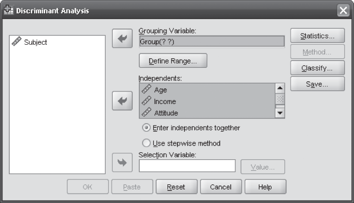
Figure 17.4 SPSS Discriminant Analysis dialog box
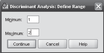
Figure 17.5 SPSS Discriminant Analysis: Define Range dialog box
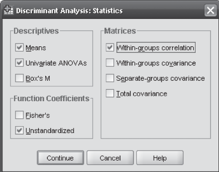
Figure 17.6 SPSS Discriminant Analysis: Statistics dialog box
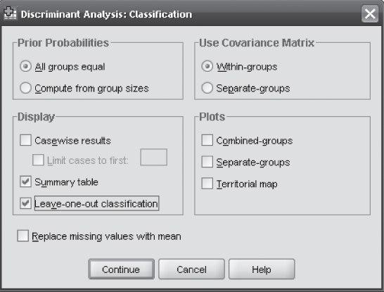
Figure 17.7 SPSS Discriminant Analysis: Classification dialog box

Figure 17.8 SPSS Discriminant Analysis: Save dialog box
17.1.7 Using Minitab for Discriminant Analysis
In the case of using Minitab for discriminant analysis, Click Start/Multivariate/Discriminant Analysis. Discriminant Analysis dialog box will appear on the screen as shown in Figure 17.9. Using Select, place Groups in the ‘Groups’ box and all the four independent variables in the ‘Predictors’ box. From ‘Discriminant Function’ select ‘Cross-Validation’ and click on Options. Discriminant Analysis - Options dialog box will appear on the screen (Figure 17.10). In this dialog box, select ‘Display of Results’ and select the fourth category, Above plus mean, std. dev., and covariance summary, and follow the routine commands, then the Minitab output will appear on the screen as shown in Figure 17.11.
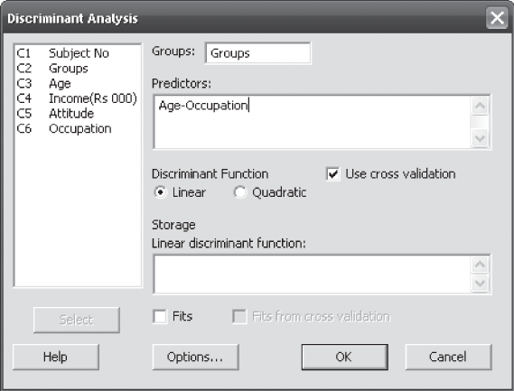
Figure 17.9 Minitab Discriminant Analysis dialog box
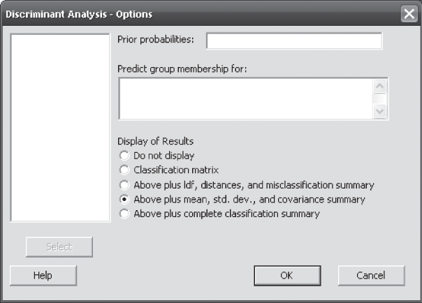
Figure 17.10 Minitab Discriminant Analysis-Options dialog box
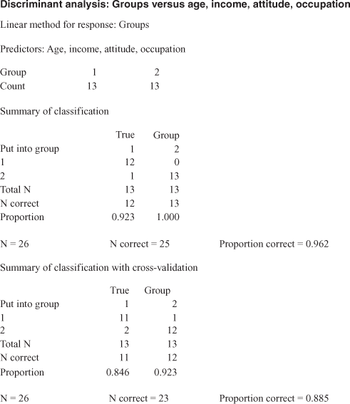
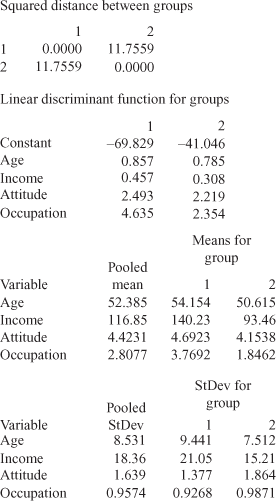

Figure 17.11 Minitab output for Example 17.1
Similar to SPSS, the Minitab output also includes ‘Summary of classification’ and ‘Summary of classification with cross-validation.’ Interpretation of this is same as discussed earlier. Linear analysis is performed when one assumes that covariance matrices are equal for all the groups. To conduct a quadratic discriminant analysis, the assumption that “covariance matrices are equal” is not made. The linear discriminant score for each group has an analogy with the regression coefficients in multiple regression analysis. The group with the largest linear discriminant function or regression coefficient contributes most to the classification of observations, which is given under the heading ‘Linear discriminant function for groups’ in the output. This part of the output indicates that for age, the highest linear discriminant function is 0.857 for Group 1, as compared with 0.785 for Group 2. This indicates that Group 1 contributes more than Group 2 to the classification of group membership.
Minitab presents descriptive statistics such as ‘mean for groups,’ ‘pooled mean,’ ‘standard deviation,’ and ‘pooled standard deviation.’ Mean indicates simple average and pooled mean is the weighted average of the means of each true group (the actual group to which an observation is classified). Standard deviation indicates simple standard deviation and pooled standard deviation is the weighted average of the standard deviations of each true group (the actual group to which an observation is classified).
The Minitab output also includes ‘covariance matrix for Group 1’ and ‘covariance matrix for Group 2.’ A covariance matrix is a non-standardized matrix, which indicates the relationship between each pair of variables. In addition, Minitab also presents ‘pooled covariance matrix’ and gives the average individual group covariance matrices element by element.
Squared distances mentioned in the ‘Summary of misclassified observations’ measure squared distances from each misclassified point to the group centroid. In the summary of misclassified observations table, ‘True group’ indicates the actual group in which a customer has been classified, ‘Pred Group’ indicates that an observation should be placed in the concerned group based on the predicted squared distances, and ‘X-val’ group indicates that using cross-validation an observation should be placed in the concerned group based on the predicted squared distances.
As discussed, the squared distance measures the distance of an observation from the group mean. ‘Squared distance pred’ and ‘Squared distance X-val’ indicates the squared distance value for each observation from each group for the result, with and without cross-validation. ‘Probability Pred’ and ‘Probability X-val’ indicates the predicted probability of a customer being placed in each group based on the result with and without cross-validation.
17.2 Multiple Discriminant Analysis
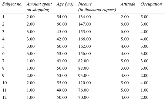
In recent years, the technique of multiple discriminant analysis has been in widespread use in both theoretical and application-oriented marketing studies.6 To understand the concept of multiple discriminant analysis, Example 17.1 can again be used with some modifications. Suppose the company has collected data from three more customers. Of the 39 customers, 27 are placed in the analysis sample and the remaining 12 are placed in the hold-out sample. As can be seen from the last column of Table 17.3, customers are divided into three categories, high, medium, and low, based on the amount they spent in shopping. In Table 17.4; 3, 2, and 1 indicate high, medium, and low amount spent on shopping. We are supposed to perform a discriminant analysis to identify the variables that are relatively better in discriminating between high, medium, and low amount spent on shopping. We will be repeating the process of discriminant analysis for multiple discriminant analysis as below.
TABLE 17.3 Data obtained for the garment company (hold-out sample)
Perform a discriminant analysis to identify the variables that are relatively better in discriminating between the satisfied and the not satisfied consumers.
Table 17.4 Data (recollected) obtained for the garment company (analysis sample)
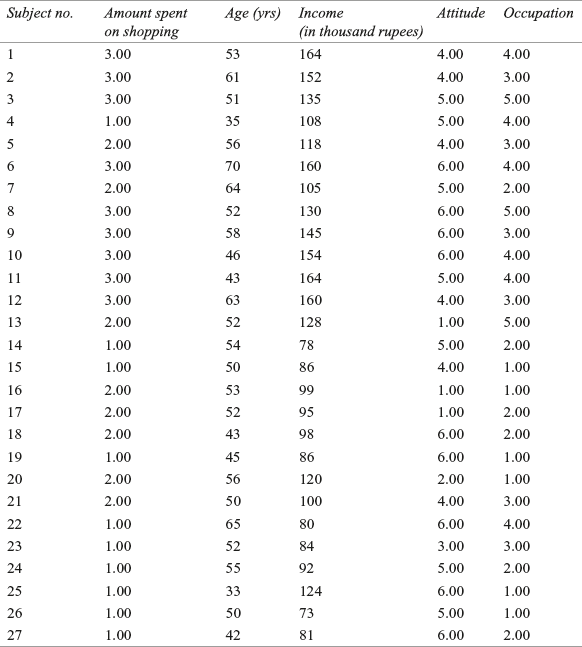
17.2.1 Problem Formulation
The problem has already been formulated with some modifications in Example 17.1. In the analysis sample, there are 27 customers, and in the hold-out sample, there are 12 customers. Through discriminant analysis, we will examine whether customers who spend high, medium, and low amounts on shopping can be differentiated in terms of age, income, attitude, and occupation. Table 17.4 shows analysis sample with 27 customers and Table 17.5 shows hold-out sample with 12 customers.
Table 17.5 Data (recollected) obtained for the garment company (hold-out sample)
SPSS output [Figure 17.12(a)–(l)] for Example 17.1 with one subject added in the analysis sample and dividing the customers into three categories based on the amount spent by them in shopping is shown in Figure 17.12.
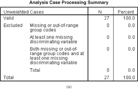
Figure 17.12 (a) Analysis case processing summary table
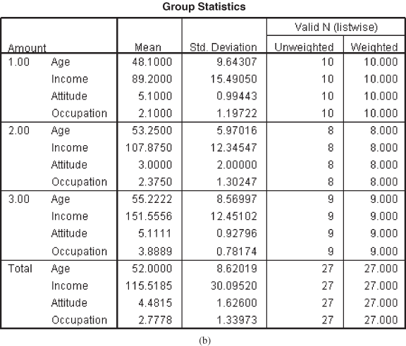
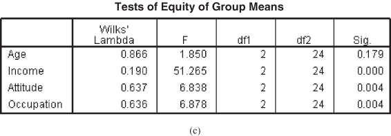
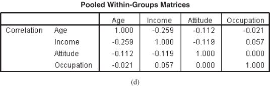
Figure 17.12 (b) Group statistics table, (c) Test of equity of group means table, (d) Pooled within-group matrices table
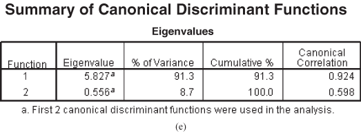
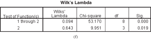
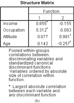


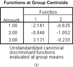
Figure 17.12 (e) Eigenvalues table, (f) Wilks’ Lambda table, (g) Standardized canonical discriminant function coefficients, (h) Structure matrix table, (i) Canonical discriminant function coefficients table, (j) Function at group centroids table
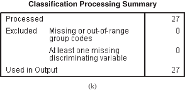
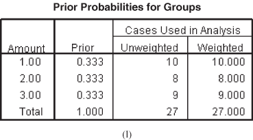
Figure 17.12 (k) Classification processing summary table, (l) Prior probabilities for groups table
17.2.2 Computing Discriminant Function Coefficient
In Example 17.1, only one discriminant function was created because there were only two groups (levels) related to the criterion variable. In multiple discriminant analysis, if there are G groups, G−1 discriminant functions can be created if the number of predictor variables is larger than this quantity. In other words, in a discriminant problem with k predictors and G groups, it is possible to create either G−1 or k discriminant functions, whichever has a lesser value.
In multiple discriminant analysis, if there are G groups, G − 1 discriminant functions can be created if the number of predictor variables is larger than this quantity. In other words, in a discriminant problem with k predictors and G groups, it is possible to create either G − 1 or k discriminant functions, whichever has a lesser value.
In our case, there are three groups and four predictors in the discriminant problem. Thus, smaller of 3−1 or 4, that is, two discriminant functions can be created. As exhibited in Figure 17.12(e), for the first function, the associated eigenvalue is 5.827 and this function contributes to 91.3% of the explained variance. For the second function, the associated eigenvalue is 0.556 and this function contributes to 8.7% of the explained variance. It can be noted that for the second function, the eigenvalue is smaller when compared with the first function and hence, the first function is likely to be superior than the second function.
17.2.3 Testing Statistical Significance of the Discriminant Function
To test the null hypothesis of equal group centroids, both the functions must be considered simultaneously. Figure 17.12(f) exhibits Wilks’ lambda table. In the first column of this figure, that is, “Test of function(s)”, Columns 1 to 2 indicate that no function has been removed. For this, Wilks’ lambda value is calculated as 0.094. After χ2 transformation, value of χ2 statistic is calculated as 53.170 with eight degrees of freedom. The corresponding p value is significant, which indicates that the two functions taken together significantly discriminate among the three groups—high, medium, and low. In the first column of the second row of Figure 17.12(f), “2” indicates that when the first function is removed, Wilks’ lambda associated with the second function is 0.643. After χ2 transformation, value of χ2 statistic is calculated as 9.951 with three degrees of freedom. The corresponding p value is significant, which indicates that the second function does contribute significantly to group difference.
17.2.4 Result (Generally Obtained Through Statistical Software) Interpretation
The interpretation of the result for multiple discriminant analysis is almost the same with some additional plots and extraction of two functions. The structure matrix exhibited in Figure 17.12(h) is within-group correlation of each predictor variable with the canonical function. An asterisk mark associated with each variable exhibits its largest absolute correlation with one of the functions. As can be seen from Figure 17.12(h), income and occupation have the strongest correlation with Function 1 and attitude and age have the strongest correlation with Function 2.
The interpretation of the result for multiple discriminant analysis is almost the same with some additional plots and extraction of two functions.
Figure 17.13 is SPSS-combined group plot for multiple discriminant analysis. From the figure, it can be seen that Group 3 has the highest value on Function 1. Group 1 has the lowest value on Function 1 with Group 2 in the middle. Group 3 is the group that spends highest on shopping. We have already discussed that income and occupation are predominantly associated with Function 1. It indicates that those with higher income and higher occupation are likely to spend more amounts on shopping. An examination of group means on income and group means on occupation strengthens this interpretation.
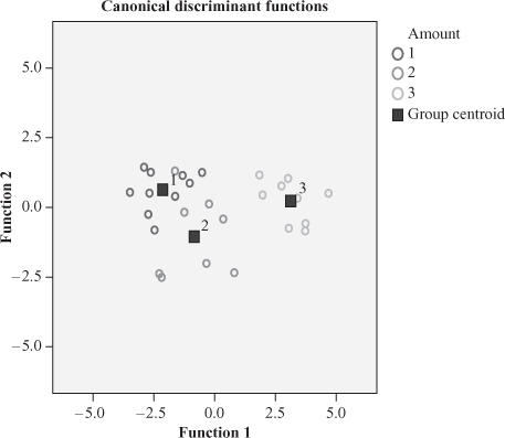
Figure 17.13 SPSS combined group plot for multiple discriminant analysis
From Figure 17.12(j), it can be seen that Group 1 has the highest value on Function 2 and Group 2 has the lowest value on Function 2. Function 2 is predominantly associated with attitude and age. Group 1 is higher in terms of attitude and age as compared with Group 2. Even with low income, Group 1 has got more positive attitude for shopping. From Figure 17.12(b) (group statistics table), we can see that the age of customers in Group 1 is lesser than the age of customers in Group 2. It seems that because of their young age, the customers in Group 1 are enthusiastic about shopping but less income is forcing them not to spend much on shopping.
Figure 17.14 shows SPSS-produced territorial plot for multiple discriminant analysis. In a territorial map, group centroid is indicated by an asterisk. In the plot, numbers corresponding to groups are scattered to exhibit group boundaries. Group 1 centroid is bounded by Number 1, Group 2 centroid is bounded by Number 2, and Group 3 centroid is bounded by Number 3.
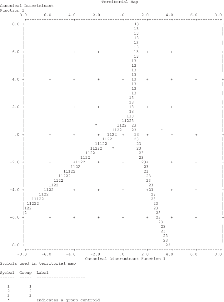
Figure 17.14 SPSS-produced territorial plot for multiple discriminant analysis
17.2.5 Concluding Comment by Performing Classification and Validation of Discriminant Analysis
Figure 17.15 is the classification result table. The hit ratio is the sum of the diagonal elements 26 (i.e., 10 + 7 + 9 = 26) divided by the total number of elements. Hence, the hit ratio can be computed as 26/27 = 0.9629. From Figure 17.15, a line can be seen as a part of the SPSS output that “96.3% of the original grouped cases correctly classified.” This 96.3% is the hit ratio. The percentage of chance qualification is 1/3 = 0.33. As discussed, classification accuracy obtained from discriminant analysis is 25% greater than that obtained from chance; validity of the discriminant analysis is judged as satisfactory. In our case, this figure is obtained as 0.58 (0.33 + 0.25). The obtained hit ratio is 96.3%, which is greater than 0.58; hence, validity of the discriminant analysis is judged as satisfactory. Leave-one-out-classification (cross-validation) indicates that 77.8% of the cases are correctly classified.
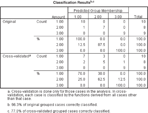
Figure 17.15 SPSS produced classification results table
The classification matrix of the hold-out sample (Figure 17.16) indicates that 91.7% of the cases are correctly classified and cross-validation indicates that 75% of the cases are correctly classified.
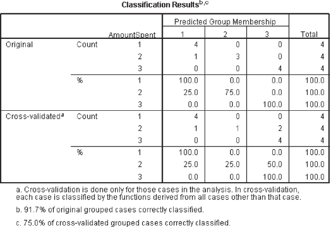
Figure 17.16 SPSS classification results table for hold-out sample (multiple discriminant analysis)
17.3 Logistic (or Logit) Regression Model
Logistic regression model, or logit regression model, somewhere falls in between multiple regression and discriminant analysis. In logistic regression, like in discriminant analysis, dependent variable happens to be a categorical variable (not a metric variable). As different from discriminant analysis, in a logistic regression model, dependent variable may have only two categories which are binary and are coded as 0 and 1 (in case of a binary logit model). So, logistic regression seems to be an extension of multiple regression where there are several independent variables and one dependent variable which has got only two categories (in case of a binary logit model). However, regression equation has got some different meaning in logistic regression. In a standard regression model, weights associated with independent variables are being used to predict a value of dependent variable, which happens to be metric in nature. On the other hand, in a logistic regression model, the value being predicted happens to be a probability value and it falls in between 0 and 1. Over the years, logistic regression model has gained popularity in the field of marketing research. Following are some of the reasons for the popularity of logistic regression models among the researchers:
- Logistic regression does not assume a linear relationship between the dependent and independent variables;
- Independent variables need not to be interval;
- Logistic regression does not require that the independents be unbounded; and
- Normally distributed error terms are not assumed7
Note that logistic regression model graph is not linear in pattern. It is somewhat S-shaped and obviously generates predictions that are always in between 0 and 1.
Logistic regression seems to be an extension of multiple regression where there are several independent variables and one dependent variable which has got only two categories (in case of a binary logit model).
17.3.1 Steps in Conducting Logistic Regression
Logistic regression can be executed following a four-step procedure: problem formulation; fitting of logistic regression model; testing model fit and statistical significance of the coefficients; and validation of the model. Figure 17.17 exhibits four steps in conducting logistic regression.
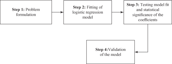
Figure 17.17 Four steps in conducting logistic regression
17.3.1.1 Problem Formulation
In order to understand logistic regression probabilities, it is important to have a clear comprehension of the odds and the logarithm of odds. In simple words, probability is the likelihood or chance that a particular event will or will not occur. The theory of probability provides a quantitative measure of uncertainty or likelihood of occurrence of different events resulting from a random experiment, in terms of quantitative measures ranging from 0 to 1.8 A probability of 0.25 for purchase intention indicates that the possibility of purchase is 25%. This also indicates that probability of non purchase is 75%. The concept of ‘odd’ indicates a ratio of the probability of occurrence and nonoccurrence of an event. Hence, in this case, odds can be defined as:
![]()
Logistic regression can be executed following a four-step procedure: problem formulation; fitting of logistic regression model; testing model fit and statistical significance of the coefficients; and validation of the model.
Concept of ‘odd’ indicates a ratio of the probability of occurrence and nonoccurrence of an event.
In a logit regression model, a construct known as logit is being created. This logit is the natural logarithm of odds discussed above. So, 25% chance of purchase has a logit as described below:
![]()
We know that probability lies in between 0 and 1, but odds can be greater than one. For example, in the above example, we take 75% chance of purchase, then, the chance of non-purchase will become 25%. In this case, odds value will be computed as three, which is greater than one. Logit in a logistic regression is a natural logarithm of the odds.
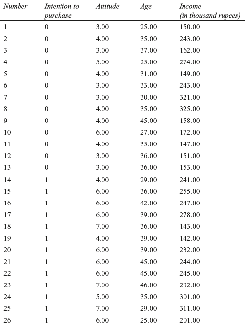
In order to understand logistic regression well, let us formulate a problem. Table 17.6 indicates the intention to purchase a product in terms of purchase or non-purchase. Data was collected from 26 respondents. Their purchase is dependent upon three independent variables – attitude for shopping, age and income. We will have to build a logistic regression model where dependent variable intention to purchase has two categories 0 and 1. The objective of developing a logistic model is to estimate the probability of purchase as a function of attitude, income and age. All the independent variables are metric in nature. Logistic regression model has also got the capacity of including some non metric independent variables.
17.3.1.2 Fitting of Logistic Regression Model
In Chapter 16, we have discussed that a multiple regression equation with one dependent variable (metric) and many independent variables will look like as below:
![]()
Table 17.6 Data pertaining to intention to purchase, attitude towards shopping, age and income
For our problem, the above regression equation can be written as:
![]()
Evidently, in a simple multiple regression model intention to purchase is a function of a constant added by coefficient times of the amount of independent variables attitude, age and income. Logistic regression presents a different concept as dependent variable has only two categories. In case of a logistic regression, we will examine whether or not there will be a purchase instead of a case of simple multiple regression where we examine purchase as a linear combination of three independent variables taken for the study. In a logistic regression case, there will be only two possible outcomes: purchase and no-purchase. So, in case of a logistic regression model, the probability of purchase will be modeled as below:
![]()
or ![]()
or ![]()
Note that ![]() is nothing but the odds discussed in the beginning of this section. Hence, odds can be computed as:
is nothing but the odds discussed in the beginning of this section. Hence, odds can be computed as:
![]()
Symbolically, if we take ![]() as the probability of success (purchase) and
as the probability of success (purchase) and ![]() as the probability of failure (no-purchase) and first independent variable attitude as
as the probability of failure (no-purchase) and first independent variable attitude as ![]() , second independent variable age as
, second independent variable age as ![]() and third independent variable income as
and third independent variable income as ![]() then above described equation will look as:
then above described equation will look as:
![]()
or ![]()
or ![]()
or ![]()
In a generalized form, above equation can be written as

In a logistic regression model, ![]() may vary from
may vary from ![]() to
to ![]() but
but ![]() will always lie between 0 and 1. Logistic regression model can be developed in a similar way as the simple multiple liner regression model can be developed allowing some of the independent variables to exhibit quadratic effect and even allowing some dummy independent variables in the model.
will always lie between 0 and 1. Logistic regression model can be developed in a similar way as the simple multiple liner regression model can be developed allowing some of the independent variables to exhibit quadratic effect and even allowing some dummy independent variables in the model.
In a logistic regression model ![]() may vary from
may vary from ![]() to
to ![]() but
but ![]() will always lie between 0 and 1.
will always lie between 0 and 1.
We have discussed in chapters 15 and 16, a method of least square as the method which minimizes the sum of squared errors of prediction for estimating parameters. In the assumptions of regression topic, we discussed the assumption of normality of error which clearly assumes errors to be normally distributed. In other words, errors in liner regression can take any value. Logistic regression presents a different scenario where errors can take only two values. If ![]() , the error is
, the error is ![]() and if
and if ![]() , the error is
, the error is![]() . So, in this case, parameters are estimated in such a way so that the predicted value of
. So, in this case, parameters are estimated in such a way so that the predicted value of ![]() will be close to 0 when
will be close to 0 when ![]() and close to 1 when
and close to 1 when![]() .
.
17.3.1.3 Testing Model Fit and Statistical Significance of the Coefficients
We can see from Figure 17.18 that the output starts from Block 1. SPSS output by default includes Block 0. Block 0 is the model that includes only intercept in the model. Researchers have a little or no interest in interpreting this model as it is based on the inclusion of intercept only ignoring the independent variables of the model. We will start our discussion from Block 1 model, which includes independent variables in the model.
Figure 17.18(a) exhibits Omnibus Tests of Model Coefficient for logit regression. The model indicates whether all the variables have been included in the logit regression equation or not. Step is the stepwise increase in the model fit. Block indicates that all the variables have been included in the current block. Figure also contains a chi-square value and its significance. We can see that for step, block and model, the chi-square values are same. The values are same because we have used enter method of regression and we have not used stepwise logistic regression or blocking. Chi-square value tests the hypothesis that the overall model is statistically significant or not. So, null hypothesis actually is the probability of obtaining the chi-square value if all the independent variables taken together will be having no impact on dependent variable. From the figure, we can see that the model is statistically significant because![]() corresponding to the model is less than 0.05 (or less than 0.01).
corresponding to the model is less than 0.05 (or less than 0.01).
Figure 17.18(b) shows Model Summary as a part of logit regression model output. The first part of this figure is −2 Log likelihood. This value indicates how well the model fits the data. Smaller value of this statistic is always desired. In fact, smaller the value of this statistic better the model is. The statistic is actually used to test the overall significance of the model. The difference between −2 Log likelihood for a null hypothesis model (a model where all the coefficient values are set as zero) and a best fit model is chi square distributed with degrees of freedom equivalent to the number of independent variables included in the model. This difference is indicated by model chi square as exhibited in Figure 17.18(a). A pefect model must have a −2 Log likelihood value as zero. −2 Log likelihood value can be used to compare nested (reduced) models in different steps of stepwise regression method. For example, in stepwise regression, in a subsequent step, after inclusion of an independent variable in the model, a decreased value of −2 Log likelihood indicates improvement in the model. This is not a part of our discussion as we have taken enter as the method of regression.
First part of this figure is −2 Log likelihood. This value indicates how well the model fits the data. Smaller value of this statistic is always desired. In fact, smaller the value of this statistic better the model is.
A pefect model must have a −2 Log likelihood value as zero.
We have discussed in Chapter 16 that in case of a multiple regression model, the coefficient of multiple determination ![]() is the proportion of variation in the dependent variable y that is explained by the combination of independent (explanatory) variables. In a logistic regression model, the two measures, Cox & Snell R square and Nagelkerke R square are somewhat similar to
is the proportion of variation in the dependent variable y that is explained by the combination of independent (explanatory) variables. In a logistic regression model, the two measures, Cox & Snell R square and Nagelkerke R square are somewhat similar to ![]() of multiple regression (note that interpretation is not exactly similar to
of multiple regression (note that interpretation is not exactly similar to ![]() of multiple regression). Cox & Snell R square is designed in such a way that it cannot reach the maximum value of 1. This limitation is overcome by Nagelkerke R square which can reach a maximum value of 1. In fact, these are pseudo R-square. Researchers must be cautious in interpreting this and must not use the similar interpretation technique what we generally use for ordinary least square regression. Cox & Snell R square value as 0.539 is generally interpreted as “the three independent variables in the logit regression model taken together account for 53.9% of the explanation for why there is purchase or not.” Higher the value of R square better the model fits the data. Other than the mentioned R square many statistics are available to assess how accurately a given model fits the data. SPSS has computed Cox & Snell R square directly as this statistic presents a close resemblance with R square statistic universally used in general regression models discussed in chapters 15 and 16 of this book.
of multiple regression). Cox & Snell R square is designed in such a way that it cannot reach the maximum value of 1. This limitation is overcome by Nagelkerke R square which can reach a maximum value of 1. In fact, these are pseudo R-square. Researchers must be cautious in interpreting this and must not use the similar interpretation technique what we generally use for ordinary least square regression. Cox & Snell R square value as 0.539 is generally interpreted as “the three independent variables in the logit regression model taken together account for 53.9% of the explanation for why there is purchase or not.” Higher the value of R square better the model fits the data. Other than the mentioned R square many statistics are available to assess how accurately a given model fits the data. SPSS has computed Cox & Snell R square directly as this statistic presents a close resemblance with R square statistic universally used in general regression models discussed in chapters 15 and 16 of this book.
Higher the value of R square better the model fits the data.
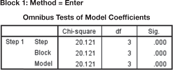
Figure 17.18(a) Omnibus tests of model coefficient
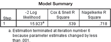
Figure 17.18(b) Model summary
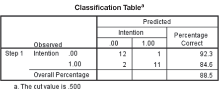
Figure 17.18(c) Classification table
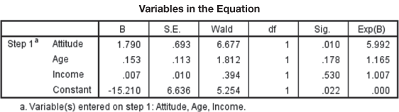
Figure 17.18(d) Variables in the equation
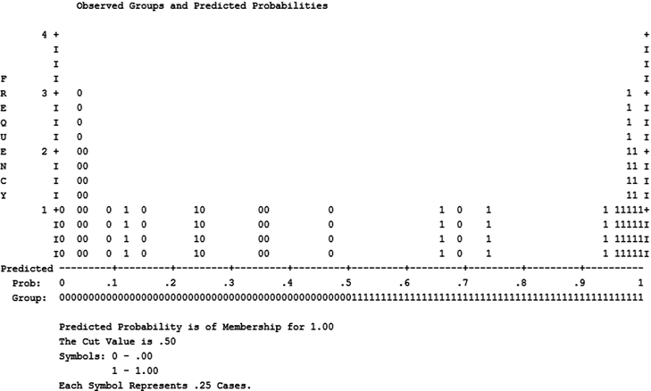
Figure 17.18(d) Variables in the equation
17.3.1.4 Validation of the Model
Figure 17.18(c) exhibits Classification Table for Intention to the purchase problem. Classification table compares the observed values of the data with predicted values for dependent variable. The table simply exhibits SPSS computation of probabilities for a particular case and places it in two predetermined catagories of dependent variable. If the computed probability is less than 0.5, SPSS places it for the first category of dependent variable (in intention to purchase example, this 0 is an indication of purchase). On the other hand, if the computed probability is greater than 0.5, SPSS places it for the second category of dependent variable (in intention to purchase example, this is 1 indicating no-purchase). From the classification table, this is very clear that for purchase (indicated by 0), ![]() of the cases are correctly classified. This is referred to as sensitivity of the prediction. In fact, this is the percentage of purchase correctly predicted. Similarly, for no-purchase (indicated by 1),
of the cases are correctly classified. This is referred to as sensitivity of the prediction. In fact, this is the percentage of purchase correctly predicted. Similarly, for no-purchase (indicated by 1), ![]() of the cases are correctly classified. This is referred to as specificity of the prediction. This is the percentage of no-purchase correctly predicted. Overall correct classification is given by
of the cases are correctly classified. This is referred to as specificity of the prediction. This is the percentage of no-purchase correctly predicted. Overall correct classification is given by ![]() . As discussed in discriminant analysis, the process of validation deals with validation sample. Like discriminant analysis, in logistic regression also we could have taken analysis sample and validation sample. Validation sample can be used for developing classification case to assess the percentage of cases correctly classified.
. As discussed in discriminant analysis, the process of validation deals with validation sample. Like discriminant analysis, in logistic regression also we could have taken analysis sample and validation sample. Validation sample can be used for developing classification case to assess the percentage of cases correctly classified.
Classification table compares the observed values of the data with predicted values for dependent variable.
Though Figure 17.18(d) is not a part of the validation process but we will discuss this here in order to maintain the sequence of discussion as exhibited in Figure 17.18 as SPSS Output for logistic regression. This actually covers statistical significance of the coefficients. Figure 17.18(d) shows variables in the equation for purchase problem. Like OLS regression, these are the coefficient values of constant and other independent variables for estimating the dependent variable with the help of independent variables. So, in case of purchase problem, the logistic regression equation will take following form:

In this equation, ![]() and
and ![]() have their usual meaning. As explained in OLS regression model in chapters 15 and 16, coefficient values indicate the amount of increase (or decrease if the sign of coefficient happens to be negative) in log odds that will be predicted by one unit increase (or decrease) in the corresponding independent variable. We can see from the above equation that the constant is −15.27 which indicates the expected values of log odds when all the independent variables are equal to zero.
have their usual meaning. As explained in OLS regression model in chapters 15 and 16, coefficient values indicate the amount of increase (or decrease if the sign of coefficient happens to be negative) in log odds that will be predicted by one unit increase (or decrease) in the corresponding independent variable. We can see from the above equation that the constant is −15.27 which indicates the expected values of log odds when all the independent variables are equal to zero.
In the third column of the Figure 17.18(d), standard errors associated with the coefficients are being given. These are actually measures of dispersion of coefficients ![]() . Standard errors can also be used for creating a confidence interval for the parameters. Fourth column of the figure indicates wald statistic and its corresponding significance (given in column 6). The wald statistic is chi square distributed with one degree of freedom if the variable is metric and the number of categories minus one if the variable is non metric.9 Wald statistic can be computed for testing the statistical significance of every variable by a simple formula
. Standard errors can also be used for creating a confidence interval for the parameters. Fourth column of the figure indicates wald statistic and its corresponding significance (given in column 6). The wald statistic is chi square distributed with one degree of freedom if the variable is metric and the number of categories minus one if the variable is non metric.9 Wald statistic can be computed for testing the statistical significance of every variable by a simple formula ![]() . In this manner, from the figure, the first value of wald statistic can be computed as
. In this manner, from the figure, the first value of wald statistic can be computed as ![]() Similarly, other values of the column can be computed.
Similarly, other values of the column can be computed.
In between, in column 5, degrees of freedom for each of the tests of the coefficients are being given. Wald statistic tests the null hypothesis that the coefficients are zero in population. From column 6 of the figure, we can see that only attitude is significant in regression model. Last column of the figure exhibits exponent values for the coefficients. For example, ![]() . Similarly, other values of the column can be computed. As different from ordinary least square regression, to assess the impact of each independent variable, we take these exponent values in to consideration. As the logistic regression model is non linear, a simple interpretation like ordinary lease square will be too generous for a researcher. For the first exponent value given in the last column of the output as 5.99, the interpretation will be “for each unit increase in attitude the likelihood of purchase will increase six times after controlling the other variables of the model.” Similarly, isolated impact of each independent variable present in the model can be catered with the help of exponent value given in the last column of the SPSS output.
. Similarly, other values of the column can be computed. As different from ordinary least square regression, to assess the impact of each independent variable, we take these exponent values in to consideration. As the logistic regression model is non linear, a simple interpretation like ordinary lease square will be too generous for a researcher. For the first exponent value given in the last column of the output as 5.99, the interpretation will be “for each unit increase in attitude the likelihood of purchase will increase six times after controlling the other variables of the model.” Similarly, isolated impact of each independent variable present in the model can be catered with the help of exponent value given in the last column of the SPSS output.
Wald statistic tests the null hypothesis that the coefficients are zero in population.
Figure 17.18(e) exhibits Observed Group and Predicted Probability Plot as a part of SPSS output. This presents a plot of predicted probabilties and observed groups. From the plot, we can see that 0 and 1 codes are being plotted on x-axis based on the predicted probability generated by the regression equation. From Figure 17.17, Logistic Regression: Options dialogue box, we can see that the classification cutoff value is by default placed as 0.5. This can be changed according to a researcher’s requirement. SPSS uses a simple rule to predict the probabilities using![]() . If
. If ![]() is greater than 0 or p is greater than 0.5, the value to be predicted as 1, otherwise it will be categorized in zero. For a perfect logistic regression model, all the 0s will lie left of all the 1s. Note that in the plot, the last line indicates ‘each symbol represents 0.25 cases’. We have 13 observation indicated by 0 and 13 observations indicated by 1 in the model. So, in the plot there should be
is greater than 0 or p is greater than 0.5, the value to be predicted as 1, otherwise it will be categorized in zero. For a perfect logistic regression model, all the 0s will lie left of all the 1s. Note that in the plot, the last line indicates ‘each symbol represents 0.25 cases’. We have 13 observation indicated by 0 and 13 observations indicated by 1 in the model. So, in the plot there should be ![]() zeros and
zeros and ![]() ones. From the plot, we can see that seven zeros are in-between predicted probability 0 and 0.1. There is one zero and a single one plotted in between predicted probability 0.1 to 0.2. Table 17.7 will make this discussion more clear.
ones. From the plot, we can see that seven zeros are in-between predicted probability 0 and 0.1. There is one zero and a single one plotted in between predicted probability 0.1 to 0.2. Table 17.7 will make this discussion more clear.
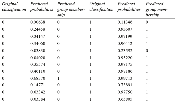
SPSS presents predicted probabilities and predicted group membership as exhibited in Table 17.7. Please note that Table 17.7 is also an explanation of Figure 17.18(c) and Figure 17.18(e). Third couumn of the table exhibits that one ‘1’ was originally wrongly classified based on the predicted probabilities (92.3% correct classification). Similarly, 2 zeros were originally wrongly classified based on the predicted probabilities (84.6% correct classification). Figure 17.18(e) is a plot of predicted probabilities exhibited in columns 3 and 6 of the table.
Table 17.7 Original classification, predicted probabilities and predicted group membership for intention to purchase problem
Logistic regression model is not restricted to only two categories of dependent variable. The model can be used for more than two categories of dependent variable and in that case it is referred to as multinomial logit.
17.3.2 Using Spss for Logistic Regression
Select Analyze from the menu bar. Select Regression from the pull-down menu. Another pull-down menu will appear on the screen. Select Binary Logistics from this menu. The Logistic Regression dialogue box will appear on the screen (see Figure 17.19). Place dependent variable in the Dependent box and independent variable in the Covariates box (refer to Figure 17.19). As a next step, from this dialogue box select Options. Logistic Regression: Options dialogue box will appear on the screen. From this dialogue box, select Classification Plots and click on Continue (see Figure 17.20). The Logistic Regression dialogue box will reappear on the screen. By clicking Save on Logistic Regression dialogue box, Logistic Regression: Save dialogue box can be opened (Figure 17.21). From Predicted Values select Probabilities and Group membership. Click Continue, Logistic Regression dialogue box will reappear on the screen. Click OK, and SPSS output, as exhibited in Figure 17.18(a) to 17.18(e), will appear on the screen.
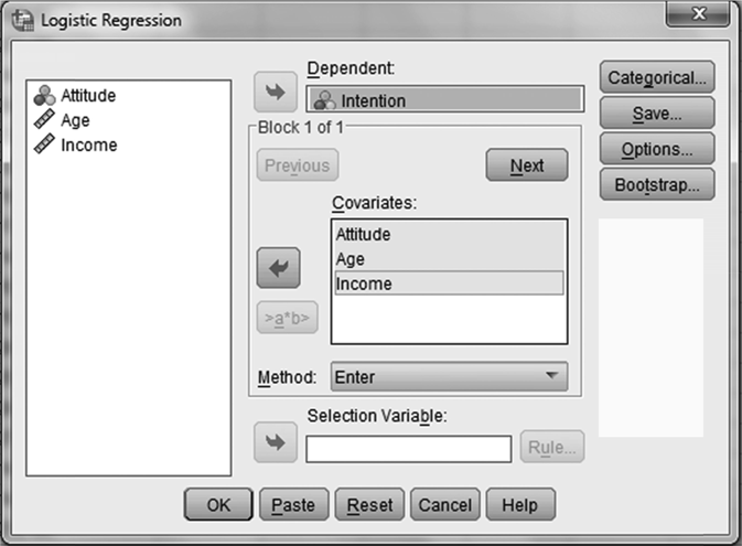
Figure 17.19 SPSS Dialogue Box for Logistic Regression
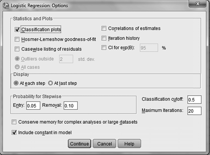
Figure 17.20 SPSS Dialogue Box for Logistic Regression: Options
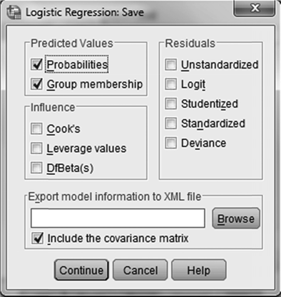
Figure 17.21 SPSS Dialogue Box for Logistic Regression: Save
17.3.3 Using Minitab for Logistic Regression
Select Stat/Regression/Binary Logistic Regression. The Binary Logistic Regression dialogue box will appear on the screen (see Figure 17.22). Select Response in response/frequency format. Place dependent variable in against Response box. Place all three independent variables in Model box. Click OK, and Minitab output (partial) for logistic regression, as exhibited in Figure 17.23, will appear on the screen. Note that Minitab presents a Log Likelihood value which if multiplied by two will present −2 Log Likelihood value of SPSS output.
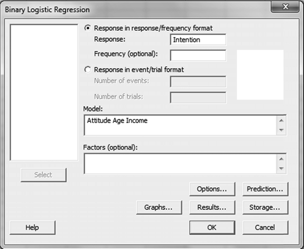
Figure 17.22 Minitab Dialogue Box for Binary Logistic Regression
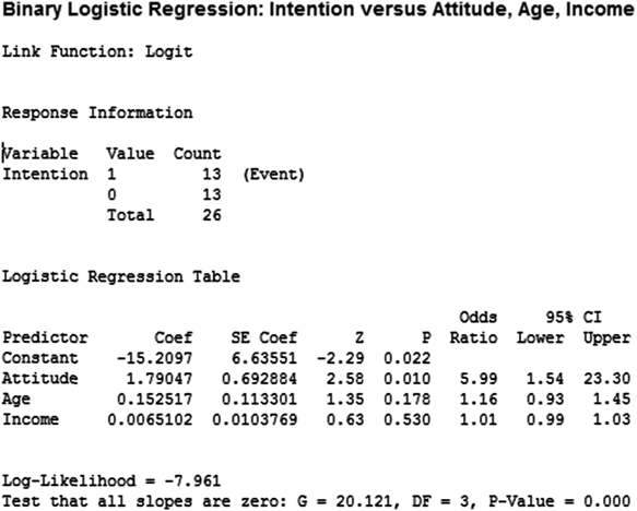
Figure 17.23 Minitab Partial Logistic regression output
Endnotes |
1. Hallaq, J. H. (1975). “Adjustment for Bias in Discriminant Analysis”, Journal of the Academy of Marketing Science, 3(2): 172–81.
2. Parasuraman, A., D. Grewal and R. Krishnan (2004). Marketing Research, pp. 514–515. Boston, MA: Houghton Mifflin Company.
3. Hair, J. F., R. P. Bush and D. J. Ortinau (2002). Marketing Research: Within a Changing Information Environment, p. 615. Tata McGraw-Hill.
4. Riveiro-Valino, J. A., C. J. Alvarez-Lopez and M. F. Marey-Perez (2009). “The Use of Discriminant Analysis to Validate a Methodology for Classifying Farms Based on a Combinatorial Algorithm”, Computer and Electronics in Agriculture, 66: 113–20.
5. Raghunathan, B. and T. S. Raghunathan (1999). “A Discriminant Analysis of Organizational Antecedents of is Performance”, Journal of Information Technology Management, 10(1–2): 1–15.
6. Sanchez, P. M. (1974). “The Unequal Group Size Problem in Discriminant Analysis”, Journal of Academy of Marketing Science, 2(4): 629–33.
7. Akinci , S., E. Kaynek, E. Atilgan and S. Aksoy (2007). “Where Does the Logistic Regression Analysis Stand in Marketing Literature? A Comparison of the Market Positioning of Prominent Marketing Journals”, European Journal of Marketing, 41(5/6):537–567.
8. Bajpai, N. (2014). Business Statistics, 2nd ed., p. 164. Pearson Education.
9. Malhotra, N. K. and S. Dash (2012). Marketing Research: An Applied Orientation, 6th ed., p.574. Pearson Education.
Summary |
Discriminant analysis is a technique of analysing data when the dependent variable is categorical and the independent variables are interval in nature. The difference between multiple regression and discriminant analysis can be examined in the light of nature of the dependent variable, which happens to be categorical, as compared with metric, as in the case of multiple regression analysis. Two-group discriminant analysis is conducted through the following five-step procedure: problem formulation, discriminant function coefficient estimation, significance of the discriminant function determination, result interpretation, and validity of the analysis determination. When categorical dependent variable has more than two categories, multiple discriminant analysis is performed.
Logistic regression model, or logit regression model, somewhere falls in between multiple regression and discriminant analysis. In logistic regression, like discriminant analysis, dependent variable happens to be a categorical variable (not a metric variable). As different from discriminant analysis, in a logistic regression model, dependent variable may have only two categories, which are binary and hence, are coded as 0 and 1 (in case of a binary logit model). So, logistic regression seems to be an extension of multiple regression where there are several independent variables and one dependent variable which has got only two categories (in case of a binary logit model). Logistic regression can be executed following a four-step procedure: problem formulation; fitting of logistic regression model; testing model fit; and statistical significance of the coefficients and validation of the model.
Key Terms |
Analysis case processing summary table, 630
Block 1, 640
Block 0, 640
Block, 640
Canonical correlation, 613
Centroids, 613
Chi-square, 614
Classification matrix, 613
Classification results table, 621
Cox & Snell R square, 640
Direct method and stepwise method, 619
Discriminant analysis model, 613
Discriminant analysis, 612
Discriminant function, 619
Discriminant scores, 614
Eigenvalue, 614
Estimation or analysis sample, 615
F values and its significance, 614
Good hit ratio, 621
Group statistics, 620
Hit ratio, 621
Hold-out or validation sample, 615
Logistic regression model, 635
Maximum chance criterion, 622
Multinomial logit, 644
Nagelkerke R square, 640
Omnibus Tests of Model Coefficient, 640
Pooled within-group correlation matrix, 614
Proportional chance criterion, 622
Structure correlation, 614
Step, 640
Unstandardized discriminant coefficients, 613
Wilks’ lambda, 614
Wald statistic, 642
Notes |
- 1. Prowess (V. 3.1): Centre for Monitoring Indian Economy Pvt. Ltd, Mumbai, accessed September 2009, reprinted with permission.
- 2. http://www.camlin.com/corporate/camlin_today.asp, accessed September 2009.
- 3. http://www.thehindubusinessline.com/2009/05/13/stories/2009051351771500.htm, accessed September 2009.
Discussion Questions |
- 1. Explain the difference between multiple regression and discriminant analysis.
- 2. What is the conceptual framework of discriminant analysis and under what circumstances can discriminant analysis be used for data analysis?
- 3. Write the steps in conducting discriminant analysis.
- 4. Write short notes on the following topics related to discriminant analysis.
(a) Estimation or analysis sample
(b) Hold-out or validation sample
(c) Pooled within-group matrices
(d) Eigenvalues
(e) Wilks’ lambda table
(f) Standardized canonical discriminant function coefficients
(g) Structure matrix table
(h) Canonical loadings or discriminant loadings
(i) Canonical discriminant function coefficients table
(j) Unstandardized coefficient
(k) Classification processing summary table
(l) Hit ratio
- 5. What is the conceptual framework of multiple discriminant analysis and under what circumstances can multiple discriminant analysis be used for data analysis?
- 6. What are the steps in performing logit analysis?
- 7. Establish a difference between discriminant analysis and logit analysis.
Case Study |
Case 17: Emami Limited: Emerging as a Well-Diversified Business Group
Introduction
The inception of Emami Group took place way back in mid-seventies when two childhood friends, Mr R. S. Agarwal and Mr R. C. Goenka, left their high profile jobs with the Birla Group to set up Kemco Chemicals, an ayurvedic medicine and cosmetic manufacturing unit, in Kolkata in 1974. In 1978, this young organization has taken over a 100-year-old company, Himani Ltd (incorporated as a private limited company in 1949), with brand equity in Eastern India. It was a highly risky decision to buy a sick unit (Himani Ltd) and was difficult to turn it into a profitable organization. Ultimately, this risky decision was proven to be a turning point for the organization. In the year 1984, the company launched its first flagship brand “Boroplus antiseptic cream,” followed by many successful brands in the following years. In 1995, Kemco Chemicals, the partnership firm was converted into a public limited company under the name and style of Emami Ltd. In 1998, Emami Ltd was merged with Himani Ltd and its name was changed to Emami Ltd as per fresh certificate of incorporation dated September 1998.1 Table 17.01 lists sales and profit after tax (in million rupees) of Emami Ltd from 1994–1995 to 2007–2008.
Looking for Consolidation of the Business Through Brand Extension, Penetration in New Markets, and Launching Fresh Categories of Products
Emami has also planned to launch a Rs 4000 million biofuel project in Ethiopia. In an interview to The Financial Express, the directors of Emami Group Mr Aditya V. Agarwal and Mr Manish Goenka discussed about the biofuel and inorganic growth options. They said, “We are always on the lookout of financially viable acquisitions. We may even consider acquiring companies outside India, particularly in underdeveloped and developing countries. Our revenue from international operations is currently around Rs 1000 million. We expect this to grow to Rs 3000 million in 3 years and about Rs 7000 millions in 5 years.
TABLE 17.01 Sales and profit after tax (in million rupees) of Emami Ltd from 1994–1995 to 2007–2008
We are contemplating some regional brand acquisition. There are some heritage brands in Bengal that offers immense growth potential. After the Zandu acquisition, we together have the portfolio of around 350 brands. A restructuring of the brand portfolio is underway, and we will clearly define the exact role and positioning of each brand. For instance, each brand will be categorized as natural, ayurvedic, or synthetic. We will also launch new products. We also plan to launch a men’s range, baby range including soap, talc and oil and further expand our FMCG business via brand extensions, penetration in new markets and fresh categories.” The directors are optimistic about the future of biofuel business.2
The Emami group has plans to consolidate its fast-moving consumer goods (FMCG) business and realty business. It has taken a decision to bring its FMCG business under the flagship of the group Emami and realty company under the separate company Emami infrastructure. Mr N. H. Bhansali, CFO and President of Emami Ltd, highlighted the company’s policy as “consolidation of FMCG business under one company, Emami, will also ensure various operational synergies, improve profitability, and lead to optimum utilization of the existing manufacturing facilities. Sales and distribution channels of two companies will also get integrated.”3
Emami has unveiled Rs 55,000 million investment plan for its flagship Emami and other group companies. This is a move to make the group a Rs 60,000 million group over 2 years (The plan was unveiled in 2009). Talking about the plan, Mr R. S. Agarwal, Executive Chairman of the company, said, “Following the merger of Zandu Pharmaceuticals Works with Emami, we intend to re-launch the Zandu products as well as launch new products in the hair and skincare segment to boost earnings. These initiatives along with our attempt to streamline the operation of the two companies post-merger will require a lot of investment.”4
Some Growth Drivers of Indian FMCG Industry
In India, some distinct factors seem to have generated a ray of great hope for the FMCG industry. The number of households using FMCG products is increasing day by day. The income of rural India is on increase because of increased irrigation facilities. Higher income and heavy television advertisements have fostered the use of branded products. Increase in disposable income, high aspirations of individuals, and higher spending on personal hygiene are also increasing. Few demographic factors, such as a large number of decisive youths, are in favour of FMCG companies. The retail sector in India is dominated by more than 12 million small outlets (one of the highest in the world in any single country) providing a large base for FMCG companies. The government’s initiatives on infrastructure development in rural areas are supportive in providing untapped market of rural India. The development of new products in providing a large range to consumers will also enhance the market for FMCG.5 Emami Ltd has already unveiled its plan to provide all these favourable factors and become a more than Rs 60,000 million company in a couple of years.
Emami Ltd has plans to launch few men’s range products. Assume that the company wants to conduct a research programme to understand the influence of various independent variables on three types of customer groups: urban customers, rural customers, and semi-rural customers, then a researcher collects relevant independent variables from the literature and develop a discriminant model to identify the discriminating power of these independent variables on the three categories of the dependent variable, “type of customers.” Create two categories of dependent variable “type of customers” without changing independent variables. Perform logit analysis described in the chapter and discuss the obtained result.
Notes |
- 1. http://www.emamiltd.in/about.asp?detail=history
- 2. http://www.financialexpress.com/printer/news/499390
- 3. http://economictimes.indiatimes.com/articleshow/ 4685147.cms?prtpage=1
- 4. http://economictimes.indiatimes.com/articleshow/ 4888190.cms?prtpage=1
- 5. Prowess (V. 3.1): Centre for Monitoring Indian Economy Pvt. Ltd, Mumbai, accessed September 2009, reprinted with permission.