
Introduction
In the previous chapter, we built an R package using Rcpp. Moreover, using CodeBlocks, we established the infrastructure for developing and building our ABI-compliant library of statistical functions (libStatsLib.a), which we linked into our R package (StatsR.dll). For the moment, we have only used a single function, library_version (defined in StatsR.cpp). We used this to illustrate the build process and to test the communication between R and C++.
In this chapter, we look in detail at how to expose the functionality of the underlying statistical library. We first look at the descriptive statistics and linear regression functions. Then we examine RcppModules in the context of the statistical test classes. The final part of this chapter looks at using the component with other R packages. We cover testing, measuring performance, and debugging. The chapter ends with a small Shiny app demonstration.
The Conversion Layer
In the C++/CLI wrapper (Chapter 3), we spent some time developing an explicit conversion layer, where we put the functions to translate between the managed world and native C++ types. The approach taken by Rcpp means that we no longer need to do this. We make use of types defined in the Rcpp C++ namespace in addition to standard C++ types, and we let Rcpp generate the underlying code that allows communication between R and C++. This interface ensures that our underlying statistical library is kept separate and independent of Rcpp.
As pointed out in the previous chapter, the Rcpp namespace is quite extensive. It contains numerous functions and objects that shield us from the basic underlying C interface provided by R. We only use a small part of the functionality, concentrating particularly on Rcpp::NumericVector, Rcpp::CharacterVector, Rcpp::List, and Rcpp::DataFrame.
Code Organization
StatsR.cpp: Contains a boilerplate Rcpp C++ function
RcppExports.cpp: Contains the generated C++ functions
Makevars.win : Contains the Windows build configuration settings
DescriptiveStatistics.cpp
LinearRegression.cpp
StatisticalTests.cpp
This is a convenient way to organize the functionality, and we will deal with each of these in turn.
Descriptive Statistics
The Code
C++ code for the DescriptiveStatistics wrapper function

The include files: Here, we #include the main Rcpp header followed by the Standard Library includes. This is followed by the #include of "Stats.h".
The comment block: Here, we document the function parameters with their name and type. We also use the @export symbol to make the R wrapper function available to other R functions outside this package by adding it to the NAMESPACE. Don’t confuse this with the Rcpp::export attribute that follows.
Attributes: We mark the function [[Rcpp::export]]. This indicates that we want to make this C++ function available to R. We have already seen an example of this with the library_version function in the previous chapter.
The wrapper function: Finally, the code itself – the R function is called get_descriptive_statistics. The first parameter is a NumericVector. The second parameter is an optional CharacterVector. If no argument is supplied, this is defaulted. The default argument is specified using the static create function. This allows us to retain the same calling semantics as the native C++ function. That is, we can call it with either one or two parameters. The get_descriptive_statistics function returns a std::unordered_map<std::string, double>, as does the underlying C++ function.
The code inside the get_descriptive_statistics function in Listing 6-1 is straightforward. We use the Rcpp function as<T>(...) to convert the incoming argument NumericVector vec (typedef’d as Vector<REALSXP>) from an SEXP (pointer to an S expression object) to a std::vector<double>. Similarly, we use Rcpp::as<T> to convert the CharacterVector keys to a vector of strings. We pass the parameters to the underlying C++ library function GetDescriptiveStatistics and retrieve the results. The results are then passed back to R using the native STL type. Under the hood, the results are wrapped as we describe in the following.
Rcpp generated code for the get_descriptive_statistics function
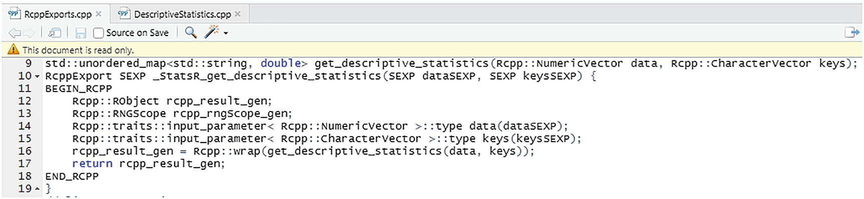
At the same time, it converts the type to an RObject and assigns the RObject pointer to rcpp_result_gen, which is then returned to R. The copy of the std::unordered_map that is returned from GetDescriptiveStatistics is destroyed, while the RObject contains a copy. It should be clear from this description that, at a slightly higher level, Rcpp::wrap provides RAII (Resource Acquisition is Initialization) around the (pointers to the) objects returned from our native C++ code. That is Rcpp::wrap provides lifetime management which simplifies the C++ wrapper code considerably.
Retrieving the R class from a C++ wrapper function
Labelled output from the get_descriptive_statistics function
Exception Handling
An example of exception handling
From Listing 6-5, we can see that if we pass in too few data points to the underlying GetDescriptiveStatistics function, the exception is reported in an informative way. Summarizing what we have seen so far, it is clear that the Rcpp framework allows us to write clean C++ code while taking care of numerous details relating to translating between R and C++.
Exercising the Functionality
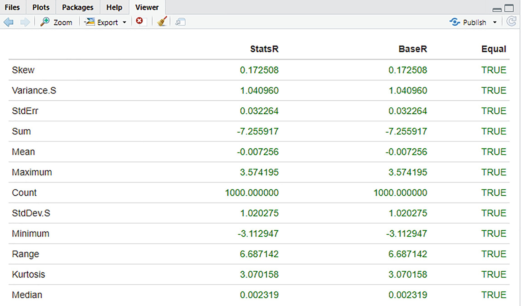
Comparison of statistics: StatsR vs. BaseR
From the table in Figure 6-1, we can immediately see that there are no numeric differences in the values produced by both libraries.
Linear Regression
The Code
Wrapper function for LinearRegression
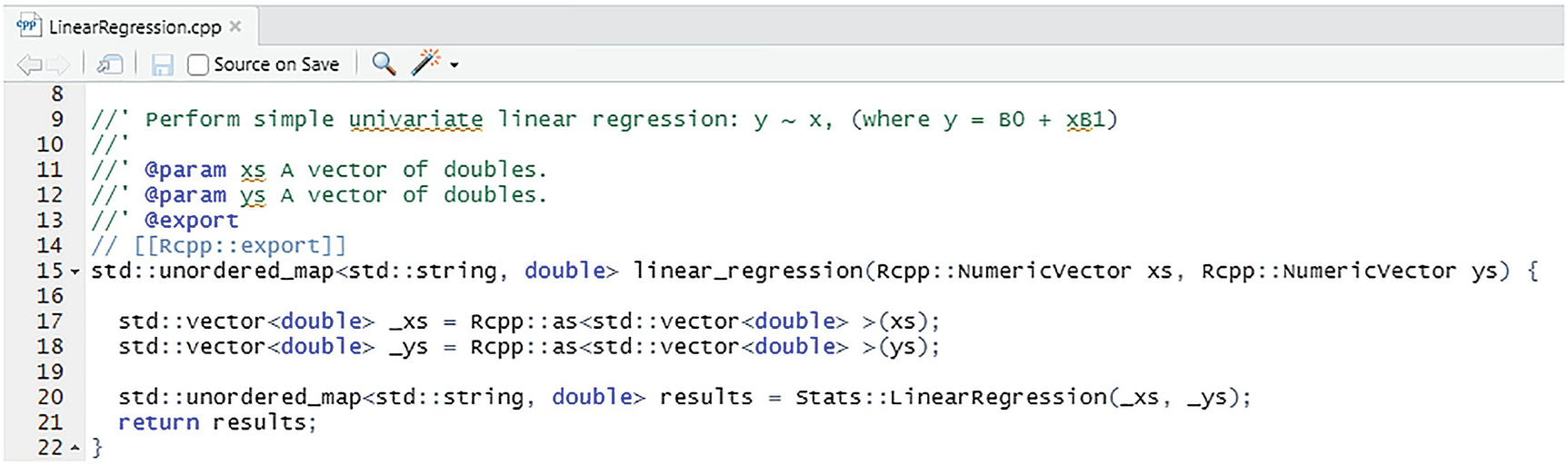
After the #includes, the function itself is declared as taking two NumericVectors and returning the results as before using std::unordered_map<std::string, double>. And as before, we use Rcpp::as<T> to copy the incoming vector to an STL type and rely on the implicit wrap to convert the results into a package of name value pairs. As discussed in the previous section, we leave the exception handling to the code generated by the Rcpp framework .
Exercising the Functionality
A simple linear model for house price prediction

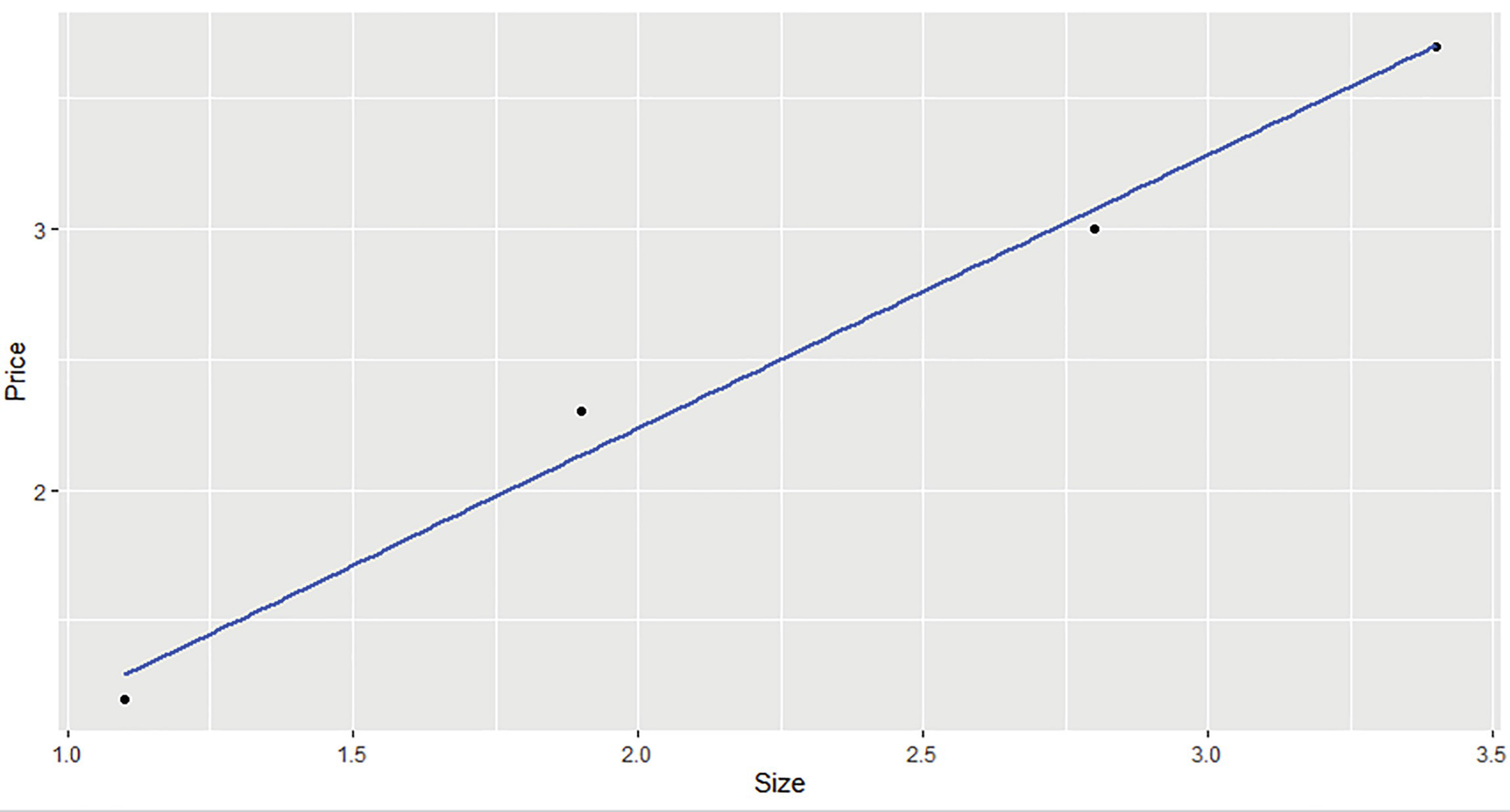
Scatterplot of house price against size
We call the wrapper function StatsR::linear_regression to obtain the model results and use the coefficients to predict a new value. Finally, we compare the results with the equivalent (but much more powerful) lm function in R. We can see that both the intercept (b0) and the slope (b1) are identical.
Using a DataFrame
Passing a DataFrame to the linear_regression function
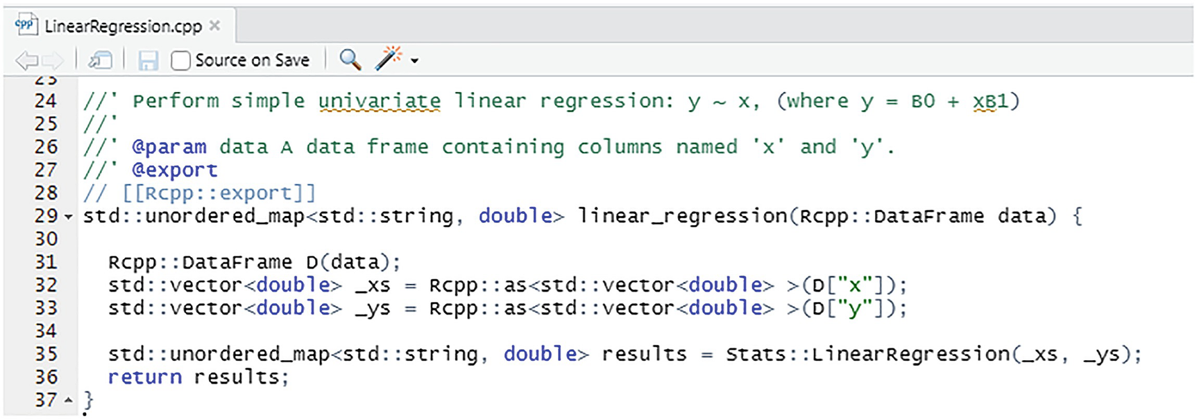
We can see from Listing 6-8 that the only difference between this function and the previous one is that we pass in a single parameter, an Rcpp::DataFrame. We assume there are columns labelled "x" and "y". If the required column names do not exist, an error is generated:
("Error in StatsR::linear_regression(data) : Index out of bounds: [index="x"].").
The only caveat with this approach is that the compiler does not permit both linear_regression functions to exist. The error from the compiler is
"conflicting declaration of C function 'SEXPREC* _StatsR_linear_regression(SEXP)' ".
It appears not to be able to distinguish the one-parameter case from the two-parameter case. We can live with this by either insisting on a single function, or renaming one of the functions. The important point here is that in the wrapper layer, you can choose how to convert and present types to users.
Statistical Tests
Functions vs. Classes
Wrapper function to perform a t-test from summary data

The code in Listing 6-9 shows the function to perform a t-test from summary input data. The wrapper function takes four doubles as arguments (double mu0, double mean, double sd, double n) and returns the results as a package of key/value pairs. In the code, we need to construct a Stats::TTest object corresponding to the summary data t-test. We use the function arguments as parameters to the constructor. In the one-sample and two-sample cases, we pass in either one or two NumericVectors which are converted to a std::vector<double> as required. These are the same type of conversions that we have seen previously. After calling test.Perform, we obtain the results set. We could check explicitly if Perform returns true or false. However, if an exception is thrown, it will be handled by the Rcpp generated code.
Rcpp Modules
As we have seen, exposing existing C++ functions and classes to R through Rcpp is quite straightforward. The approach we have adopted until now is to write a wrapper function. This interface function is responsible for converting input objects to the appropriate types, calling the underlying C++ function, or constructing an instance if it is a class, and then converting the results back to a type suitable for R. We have seen a number of examples of both usages: exposing functions and classes with wrapper functions.
In certain circumstances however, it might be desirable to be able to expose classes directly to R. If the underlying C++ class has significant construction logic, for example. We would rather expose a class-like object that can be managed by R rather than incurring the cost of constructing an instance of the class on each function call, as we do with the t-test wrapper functions. More generally, exposing classes directly allows us to retain the underlying object semantics. The Rcpp framework provides a mechanism for exposing C++ classes via Rcpp modules. Rcpp modules also allow grouping of functions and classes in a single coherent modular unit.
Exposing the TTest class via the RCPP_MODULE macro

The code in Listing 6-10 is in srcStatisticalTests.cpp. There are two parts to this code. The first part declares a C++ TTest wrapper class. This class wraps a native Stats::TTest member. The C++ wrapper class is used to perform the required translations between types. The constructors for the summary data and one-sample t-tests take the same Rcpp arguments as in the procedural wrappers and perform the same conversions we have seen before. The two-sample t-test uses an Rcpp::List object containing two numeric vectors labelled “x1” and “x2”. The methods Perform and Results are simply forwarded to the underlying native Stats::TTest instance. The design pattern is similar to a pimpl (pointer-to-implementation ) idiom or a facade or adaptor pattern.
Using the TTest class in an R script
In Listing 6-11, we create a module object by calling the Module function with the name "StatsTests". Entities inside the module may be accessed via the $ symbol. Note that in our limited example, we have only placed a single entity inside the Rcpp module. However, there is no reason why this could not also contain other classes and related functionality. In R, we instantiate our TTest class as ttest0 using new with the object name followed by the parameters. We can then use the instance ttest0 to perform the test and print the results or an error message.
Overall, RcppModules provide a convenient way both to group functionality and to expose C++ classes. We therefore have the choice of writing wrapper functions or wrapper classes, whichever suits our purposes best. This has been a brief introduction to RcppModules. There are numerous details of this approach that we have not covered here.
Testing
test_descriptive_statistics.R
test_linear_regression.R
test_statistical_tests.R
The LinearRegression test

The LinearRegression test in Listing 6-12 creates x and y values and places these in a data frame. We then call the R function lm followed by our LinearRegression function. Finally, we compare the intercept and slope coefficients.
Testing the summary t-test from data

In Listing 6-13, we only test the wrapper function as it is slightly easier to call than the class.
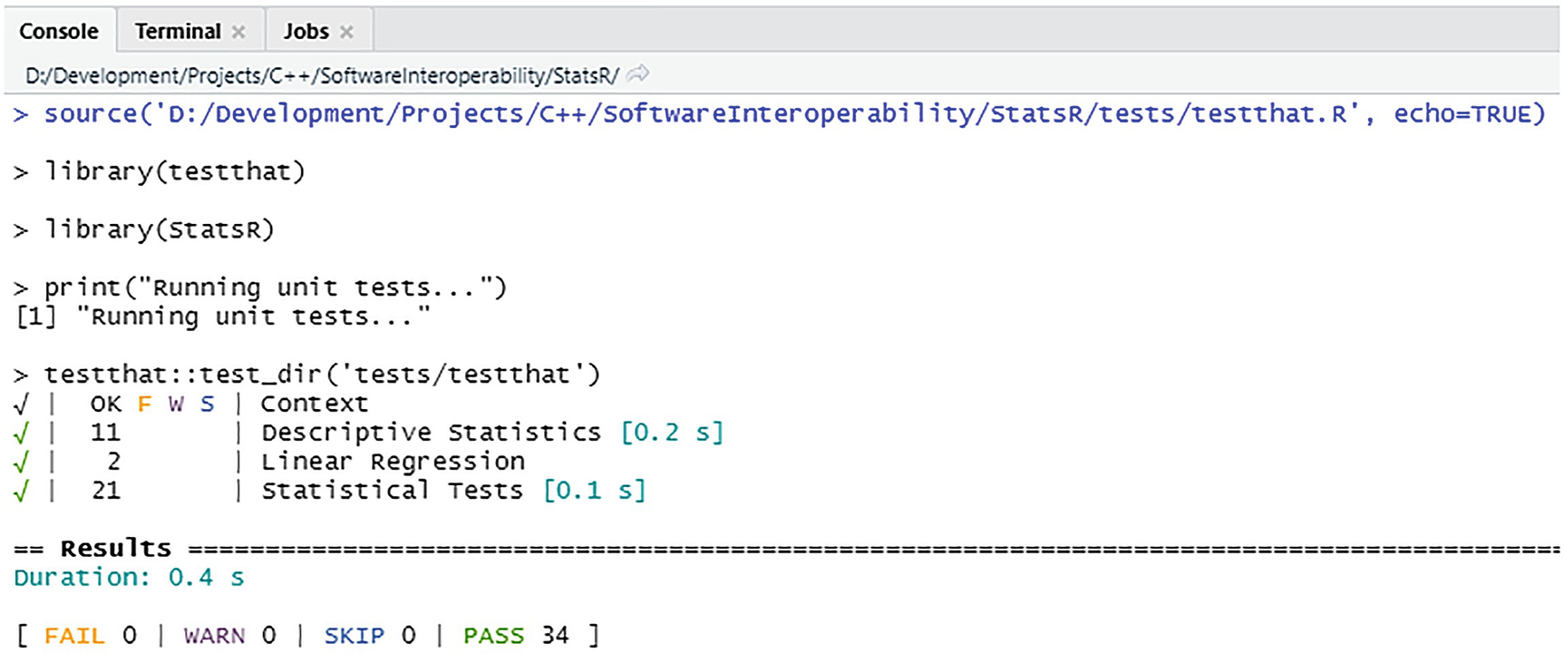
Running the test harness
The output from the test run in Figure 6-3 indicates that all the tests (34 of them) passed. There were no failures, warnings, or tests that were skipped. It also outputs the test durations.
Measuring Performance
shows Benchmark.R
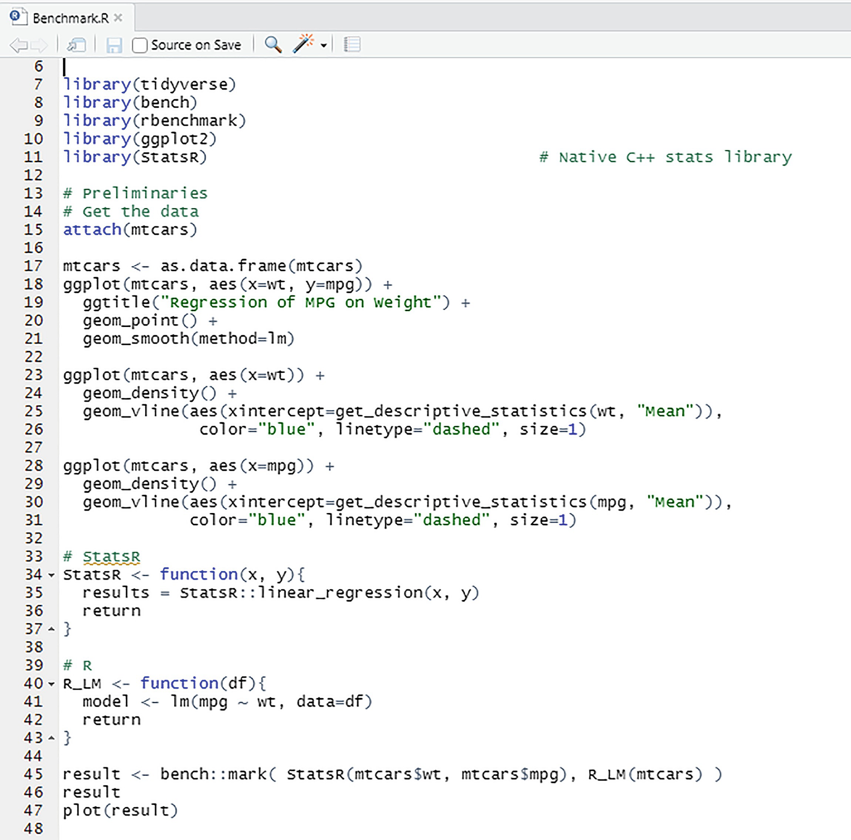

Benchmark comparison of StatsR and R lm functions
The difference in the timings is not surprising since the lm function does much more than our limited LinearRegression function.
Debugging
Navigate to the directory with the sources (SoftwareInteroperabilityStatsRsrc).
Start gdb with the Rgui as a parameter as follows: gdb D:/R/R-4.0.3/bin/x64/Rgui.exe.

A typical gdb session
This will now break into the debugger at the call location. From here we can single step through the function call (command n). However, the information from the individual function calls is quite limited, which makes debugging less useful than it should be.
Distribution Explorer

StatsR Shiny App
Displaying summary statistics
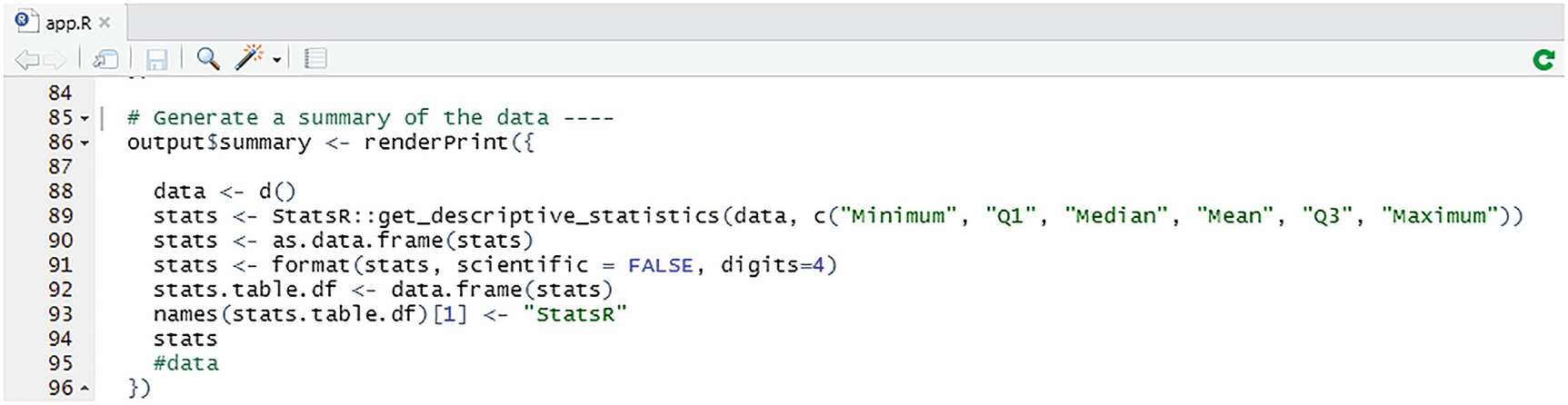
The summary statistics stats are rendered to a summary panel declared in the UI fluidPage. Once the data has been generated, we extract it as a single column NumericVector . This is passed to get_descriptive_statistics in the usual way along with the keys representing the summary statistics we want returned. Presenting the results takes a few more lines of code. First, we coerce the results into a DataFrame and format the numeric values. Then we coerce the results into a table format and return them. As can be seen, our StatsR package works, more or less seamlessly, with other R packages.
Summary
In this chapter, we have written a fully functioning R package that connects to a native C++ library. We have exposed both functions and classes from the underlying library so that they are available for use in R/RStudio. We have tested the functionality and benchmarked it.
Once we have these pieces in place (an RStudio Rcpp project, Rtools available for compiling and building, and a C++ development environment), there is nothing to stop us using any of the analytics offered in public domain C++ libraries as part of an R data analysis toolchain. We might, for example, take QuantLib (www.quantlib.org/) and use some of the interest rate curve building functionality in R. Alternatively, we might consider developing our own C++ libraries, and making these available in R. It is worth emphasizing that this goes beyond the more traditional use-case of writing small amounts of C++ code that are compiled and run inline in R with a view to improving performance. These two chapters have provided a working infrastructure for more systematic development of C++ components with the intention of making the functionality available in an R package. Rcpp makes this process seamless and takes away much of the work involved. In the next two chapters, we look at a similar situation, but in this case, our focus is on the Python language and Python clients.
Additional Resources
Rcpp is a large library. For a user-friendly introduction, I would recommend “Rcpp for everyone” at https://teuder.github.io/rcpp4everyone_en/. The official package documentation is available here: https://cran.r-project.org/web/packages/Rcpp/Rcpp.pdf. However, depending on what type of information you are looking for, there are various other sources. Apart from the book “Seamless R and C++ Integration with Rcpp” (see the References), there is a good amount of documentation covering all aspects of the package at https://github.com/RcppCore/Rcpp. Particularly recommended are the vignettes which focus on specific features of Rcpp (like RcppModules, for example). I would also recommend the Rcpp FAQ at https://cran.r-project.org/web/packages/Rcpp/vignettes/Rcpp-FAQ.pdf.
Exercises
The exercises in this section deal with incorporating the various changes we have made to the underlying codebase into the R package, and exposing the functionality via Rcpp. All the exercises use the StatsR RStudio project.
1) We extended the LinearRegression function to calculate the correlation coefficient r and r2 and added these to the results package. Confirm that the additional coefficients calculated in the LinearRegression function are displayed, and check the values.
For this, you can use the script LinearRegression.R. To check the results, use the functions cor(data) and cor(data)^2. Compare these values to the values obtained in the results package from the function StatsR::linear_regression(...). The results should be identical.
Extend the test case in test_linear_regression.R to include a check of these values.
2) The TimeSeries class has already been added to the sources, and built into the libStatsLib.a static library (see Chapter 5). Expose the MovingAverage function from the TimeSeries class. In this case, we just want to expose a procedural wrapper function. In a further exercise, we will add a class using RcppModules.
In the src directory add a new file TimeSeries.cpp. Use File ➤ New ➤ C++ File as this will create the file with the boilerplate Rcpp code.
#include the TimeSeries.h file from the Commoninclude directory.
Expose the MovingAverage method using a procedural wrapper. The following function signature is suggested:
- Implement the code:
Convert the dates to a vector of longs.
Convert the observations to a vector of doubles.
Construct an instance of the TimeSeries class.
Call the MovingAverage function and return the results.
Select Build ➤ Clean and Rebuild and check that the build (still) works without warnings or errors. Check that the file srcTimeSeries.cpp compiled correctly in the output. Check that the function is present in RcppExports.R.
- Check that the function is present in the list of functions. Use> library(pkgload)> names(pkg_env("StatsR"))
- Create some random data as follows:n = 100 # n samplesobservations <- 1:n + rnorm(n = n, mean = 0, sd = 10)dates <- c(1:n)
- Add a simple moving average function with a default window size of 5:moving_average <- function(x, n = 5) {stats::filter(x, rep(1 / n, n), sides = 1)}
- Obtain two moving averages: one from the StatsR package and one using the local function (note the window size parameter):my_moving_average_1 <- StatsR::get_moving_average(dates, observations, 5)my_moving_average_2 <- moving_average(observations, 5) # Apply user-defined function
Plot the series.
- Compare the series as they should be identical:equal <- (my_moving_average_1 - my_moving_average_2) >= (tolerance - 0.5)length(equal[TRUE])
Select Build ➤ Clean and Rebuild and check that the build works without warnings or errors. Check that the file srcStatisticalTests.cpp compiled correctly in the output. Check that the functions are present in RcppExports.R. Check that the functions are present in the list of functions.
- Use the R script StatisticalTests.R to write a script to exercise the new functions. The following script uses the same data as is used in the native C++ unit tests, the C# unit tests, and the Excel worksheet:## z-tests## Summary data z-testStatsR::z_test_summary_data(5, 6.7, 7.1, 29)# One-sample z-test dataStatsR::z_test_one_sample(3, c(3, 7, 11, 0, 7, 0, 4, 5, 6, 2))# Two-sample z-test datax <- c( 7.8, 6.6, 6.5, 7.4, 7.3, 7.0, 6.4, 7.1, 6.7, 7.6, 6.8 )y <- c( 4.5, 5.4, 6.1, 6.1, 5.4, 5.0, 4.1, 5.5 )StatsR::z_test_two_sample(x, y)
For completeness, add test cases to estthat est_statistical_tests.R.
Run the testthat.R script and confirm that all the tests pass.
Select Preview to view the changes. Select Build ➤ Clean and Rebuild. Check the file: “D:RR-4.0.3libraryStatsRhtmlStatsR-package.html”.
In StatisticalTests.cpp, write a wrapper class that contains a private member variable:
Implement the conversions required in the constructors. This is basically identical to the TTest wrapper.
- Add this class to the RcppModule:...{Rcpp::class_<ZTest>("ZTest").constructor<double, double, double, double>("Perform a z-test from summary input data").constructor<double, Rcpp::NumericVector >("Perform a one-sample z-test with known population mean").constructor<Rcpp::List >("Perform a two-sample z-test").method("Perform", &ZTest::Perform, "Perform the required test").method("Results", &ZTest::Results, "Retrieve the test results");}
In RStudio, select Build ➤ Clean and Rebuild and check that the build works without warnings or errors. Check that the file srcStatisticalTests.cpp compiled correctly in the output.
- Use the R script StatisticalTests.R to write a script to exercise the new class. The following is an example of the summary data z-test:library(Rcpp)library(formattable)moduleStatsTests <- Module("StatsTests", PACKAGE="StatsR")ztest0 <- new(moduleStatsTests$ZTest, 5, 6.7, 7.1, 29)if(ztest0$Perform()){results <- ztest0$Results()print(results)results <- as.data.frame(results)formattable(results)}else{print("Z-test from summary data failed.")}
Open TimeSeries.cpp source file.
- Add a wrapper class for the native C++ time series as follows:// A wrapper class for time seriesclass TimeSeries{public:~TimeSeries() = default;TimeSeries(Rcpp::NumericVector dates, Rcpp::NumericVector observations): _ts(Rcpp::as<std::vector<long> >(dates), Rcpp::as<std::vector<double> >(observations) ){}std::vector<double> MovingAverage(int window) {return _ts.MovingAverage(window);}private:Stats::TimeSeries _ts;};
- Define an RCPP_MODULE(TS) that describes the wrapper class, for example:Rcpp::class_<TimeSeries>("TimeSeries").constructor<Rcpp::NumericVector, Rcpp::NumericVector>("Construct a time series object").method("MovingAverage", &TimeSeries::MovingAverage, "Calculate a moving average of size = window");
Select Build ➤ Clean and Rebuild and check that the build works without warnings or errors.
- Open the file TimeSeries.R. Add code to the script that computes the same time series as previously and compares the results.moduleTS <- Module("TS", PACKAGE="StatsR")ts <- new(moduleTS$TimeSeries, dates, observations)my_moving_average_4 <- ts$MovingAverage(5)equal <- (my_moving_average_4 - my_moving_average_2) >= (tolerance - 0.5)length(equal[TRUE])