Learning Objectives
By the end of this chapter, you will be able to:
- Analyze and identify where non-linear data structures can be used
- Implement and manipulate tree structures to represent data and solve problems
- Traverse a tree using various methods
- Implement a graph structure to represent data and solve problems
- Represent a graph using different methods based on a given scenario
In this chapter, we will look at two non-linear data structures, namely trees and graphs, and how they can be used to represent real-world scenarios and solve various problems.
Introduction
In the previous chapter, we implemented different types of linear data structures to store and manage data in a linear fashion. In linear structures, we can traverse in, at most, two directions – forward or backward. However, the scope of these structures is very limited, and they can't be used to solve advanced problems. In this chapter, we'll explore a more advanced class of problems. We will see that the solutions we implemented previously are not good enough to be used directly. Due to this, we'll expand upon those data structures to make more complex structures that can be used to represent non-linear data.
After looking at these problems, we'll discuss basic solutions using the tree data structure. We'll implement different types of trees to solve different kinds of problems. After that, we'll have a look at a special type of tree called a heap, as well as its possible implementation and applications. Following that, we'll look at another complex structure – graphs. We'll implement two different representations of a graph. These structures help translate real-world scenarios into a mathematical form. Then, we will apply our programming skills and techniques to solve problems related to those scenarios.
A strong understanding of trees and graphs serves as the basis for understanding even more advanced problems. Databases (B-trees), data encoding/compression (Huffman tree), graph coloring, assignment problems, minimum distance problems, and many more problems are solved using certain variants of trees and graphs.
Now, let's look at some examples of problems that cannot be represented by linear data structures.
Non-Linear Problems
Two main categories of situations that cannot be represented with the help of linear data structures are hierarchical problems and cyclic dependencies. Let's take a closer look at these cases.
Hierarchical Problems
Let's look at a couple of examples that inherently have hierarchical properties. The following is the structure of an organization:
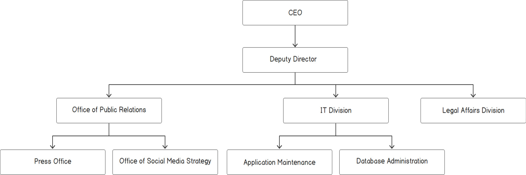
Figure 2.1: Organization structure
As we can see, the CEO is the head of the company and manages the Deputy Director. The Deputy Director leads three other officers, and so on.
The data is inherently hierarchical in nature. This type of data is difficult to manage using simple arrays, vectors, or linked lists. To solidify our understanding, let's look at another use case; that is, a university course's structure, as shown in the following figure:
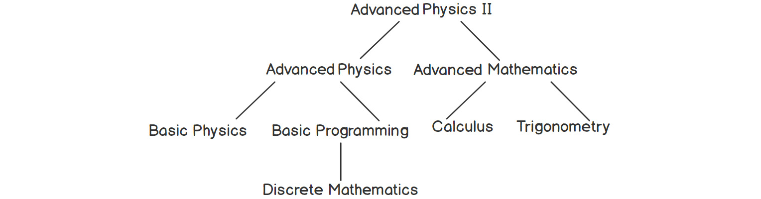
Figure 2.2: Course hierarchy in a university course structure
The preceding figure shows the course dependencies for some courses in a hypothetical university. As we can see, to learn Advanced Physics II, the student must have successfully completed the following courses: Advanced Physics and Advanced Mathematics. Similarly, many other courses have their own prerequisites.
Given such data, we can have different types of queries. For example, we may want to find out which courses need to be completed successfully so that we can learn Advanced Mathematics.
These kinds of problems can be solved using a data structure called a tree. All of the objects are known as the nodes of a tree, while the paths leading from one node to another are known as edges. We'll take a deeper look at this in the Graphs section, later in this chapter.
Cyclic Dependencies
Let's look at another complex real-world scenario that can be represented better with a non-linear structure. The following figure represents the friendship between a few people:
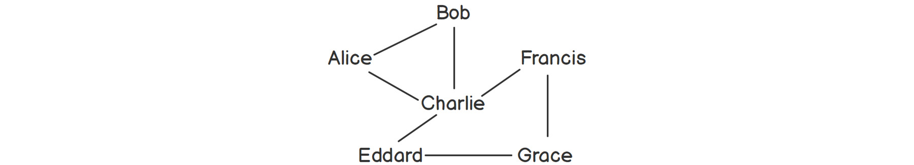
Figure 2.3: A network of friends
This structure is called a graph. The names of people, or the elements, are called nodes, and the relations between them are represented as edges. Such structures are commonly used by various social networks to represent their users and the connections between them. We can observe that Alice is friends with Charlie, who is friends with Eddard, who is friends with Grace, and so on. We can also infer that Alice, Bob, and Charlie know each other. We may also infer that Eddard is a first-level connection for Grace, Charlie is a second-level connection, and Alice and Bob are third-level connections.
Another area where graphs are useful is when we want to represent networks of roads between cities, as you will see in the Graphs section later in this chapter.
Tree – It's Upside Down!
As we discussed in the previous section, a tree is nothing but some objects or nodes connected to other nodes via a relationship that results in some sort of hierarchy. If we were to show this hierarchy in a graphical way, it would look like a tree, while the different edges would look like its branches. The main node, which is not dependent on any other node, is also known as a root node and is usually represented at the top. So, unlike an actual tree, this tree is upside down, with the root at its top!
Let's try to construct a structure for a very basic version of an organizational hierarchy.
Exercise 7: Creating an Organizational Structure
In this exercise, we will implement a basic version of the organizational tree we saw in the introduction to this chapter. Let's get started:
- First, let's include the required headers:
#include <iostream>
#include <queue>
- For simplicity, we'll assume that any person can have, at most, two subordinates. We'll see that this is not difficult to extend to resemble real-life situations. This kind of tree is also known as a binary tree. Let's write a basic structure for that:
struct node
{
std::string position;
node *first, *second;
};
As we can see, any node will have two links to other nodes – both of their subordinates. By doing this, we can show the recursive structure of the data. We are only storing the position at the moment, but we can easily extend this to include a name at that position or even a whole struct comprising all the information about the person in that position.
- We don't want end users to deal with this kind of raw data structure. So, let's wrap this in a nice interface called org_tree:
struct org_tree
{
node *root;
- Now, let's add a function to create the root, starting with the highest commanding officer of the company:
static org_tree create_org_structure(const std::string& pos)
{
org_tree tree;
tree.root = new node{pos, NULL, NULL};
return tree;
}
This is a static function just to create the tree. Now, let's see how we can extend the tree.
- Now, we want to add a subordinate of an employee. The function should take two parameters – the name of the already existing employee in the tree and the name of the new employee to be added as a subordinate. But before that, let's write another function that will help us find a particular node based on a value to make our insertion function easier:
static node* find(node* root, const std::string& value)
{
if(root == NULL)
return NULL;
if(root->position == value)
return root;
auto firstFound = org_tree::find(root->first, value);
if(firstFound != NULL)
return firstFound;
return org_tree::find(root->second, value);
}
While we are traversing the tree in search of an element, either the element will be the node we are at, or it will be in either of the right or left subtrees.
Hence, we need to check the root node first. If it is not the desired node, we'll try to find it in the left subtree. Finally, if we haven't succeeded in doing that, we'll look at the right subtree.
- Now, let's implement the insertion function. We'll make use of the find function in order to reuse the code:
bool addSubordinate(const std::string& manager, const std::string& subordinate)
{
auto managerNode = org_tree::find(root, manager);
if(!managerNode)
{
std::cout << "No position named " << manager << std::endl;
return false;
}
if(managerNode->first && managerNode->second)
{
std::cout << manager << " already has 2 subordinates." << std::endl;
return false;
}
if(!managerNode->first)
managerNode->first = new node{subordinate, NULL, NULL};
else
managerNode->second = new node{subordinate, NULL, NULL};
return true;
}
};
As we can see, the function returns a Boolean, indicating whether we can insert the node successfully or not.
- Now, let's use this code to create a tree in the main function:
int main()
{
auto tree = org_tree::create_org_structure("CEO");
if(tree.addSubordinate("CEO", "Deputy Director"))
std::cout << "Added Deputy Director in the tree." << std::endl;
else
std::cout << "Couldn't add Deputy Director in the tree" << std::endl;
if(tree.addSubordinate("Deputy Director", "IT Head"))
std::cout << "Added IT Head in the tree." << std::endl;
else
std::cout << "Couldn't add IT Head in the tree" << std::endl;
if(tree.addSubordinate("Deputy Director", "Marketing Head"))
std::cout << "Added Marketing Head in the tree." << std::endl;
else
std::cout << "Couldn't add Marketing Head in the tree" << std::endl;
if(tree.addSubordinate("IT Head", "Security Head"))
std::cout << "Added Security Head in the tree." << std::endl;
else
std::cout << "Couldn't add Security Head in the tree" << std::endl;
if(tree.addSubordinate("IT Head", "App Development Head"))
std::cout << "Added App Development Head in the tree." << std::endl;
else
std::cout << "Couldn't add App Development Head in the tree" << std::endl;
if(tree.addSubordinate("Marketing Head", "Logistics Head"))
std::cout << "Added Logistics Head in the tree." << std::endl;
else
std::cout << "Couldn't add Logistics Head in the tree" << std::endl;
if(tree.addSubordinate("Marketing Head", "Public Relations Head"))
std::cout << "Added Public Relations Head in the tree." << std::endl;
else
std::cout << "Couldn't add Public Relations Head in the tree" << std::endl;
if(tree.addSubordinate("Deputy Director", "Finance Head"))
std::cout << "Added Finance Head in the tree." << std::endl;
else
std::cout << "Couldn't add Finance Head in the tree" << std::endl;
}
You should get the following output upon executing the preceding code:
Added Deputy Director in the tree.
Added IT Head in the tree.
Added Marketing Head in the tree.
Added Security Head in the tree.
Added App Development Head in the tree.
Added Logistics Head in the tree.
Added Public Relations Head in the tree.
Deputy Director already has 2 subordinates.
Couldn't add Finance Head in the tree
This output is illustrated in the following diagram:
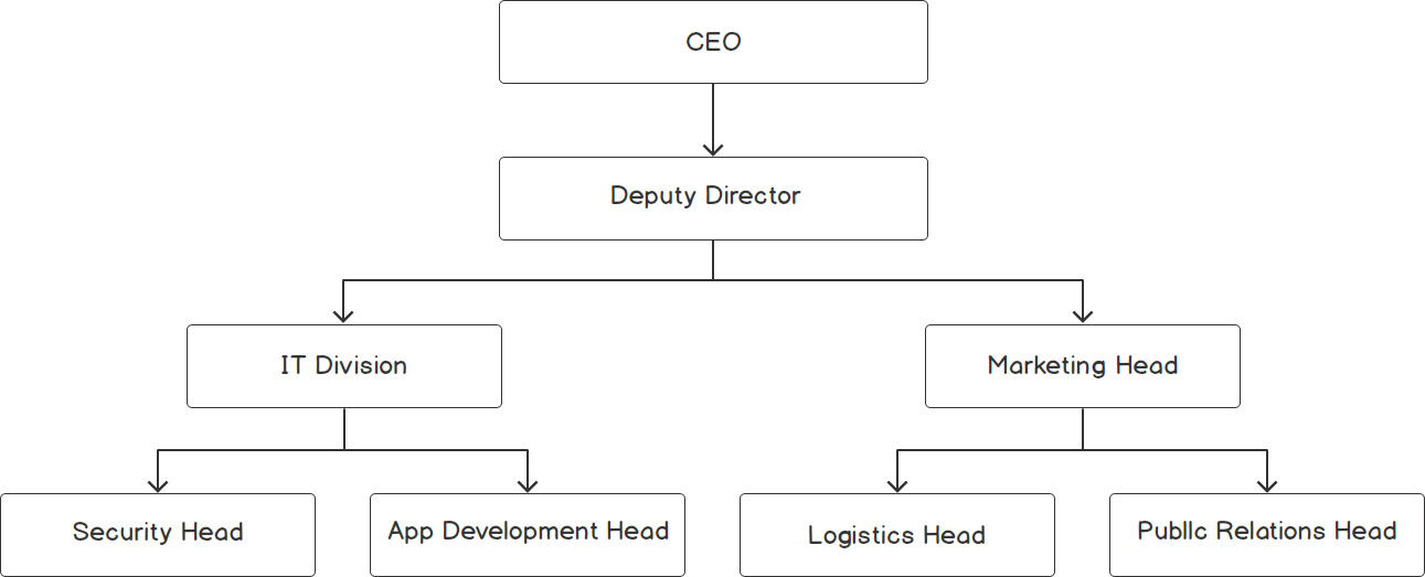
Figure 2.4: Binary tree based on an organization's hierarchy
Up until now, we've just inserted elements. Now, we'll look at how we can traverse the tree. Although we've already seen how to traverse using the find function, that's just one of the ways we can do it. We can traverse a tree in many other ways, all of which we'll look at in the following section.
Traversing Trees
Once we have a tree, there are various ways we can traverse it and get to the node that we require. Let's take a brief look at the various traversal methods:
- Preorder traversal: In this method, we visit the current node first, followed by the left child of the current node, and then the right child of the current node in a recursive fashion. Here, the prefix "pre" indicates that the parent node is visited before its children. Traversing the tree shown in figure 2.4 using the preorder method goes like this:
CEO, Deputy Director, IT Head, Security Head, App Development Head, Marketing Head, Logistics Head, Public Relations Head,
As we can see, we are always visiting the parent node, followed by the left child node, followed by the right child node. We do this not just for the root, but for any node with respect to its subtree. We implement preorder traversal using a function like this:
static void preOrder(node* start)
{
if(!start)
return;
std::cout << start->position << ", ";
preOrder(start->first);
preOrder(start->second);
}
- In-order traversal: In this type of traversal, first we'll visit the left node, then the parent node, and finally the right node. Traversing the tree that's shown in figure 2.4 goes like this:
Security Head, IT Head, App Development Head, Deputy Director, Logistics Head, Marketing Head, Public Relations Head, CEO,
We can implement this in a function like so:
static void inOrder(node* start)
{
if(!start)
return;
inOrder(start->first);
std::cout << start->position << ", ";
inOrder(start->second);
}
- Post-order traversal: In this traversal, we first visit both the children, followed by the parent node. Traversing the tree that's shown in figure 2.4 goes like this:
Security Head, App Development Head, IT Head, Logistics Head, Public Relations Head, Marketing Head, Deputy Director, CEO,
We can implement this in a function like so:
static void postOrder(node* start)
{
if(!start)
return;
postOrder(start->first);
postOrder(start->second);
std::cout << start->position << ", ";
}
- Level order traversal: This requires us to traverse the tree level by level, from top to bottom, and from left to right. This is similar to listing the elements at each level of the tree, starting from the root level. The results of such a traversal are usually represented as per the levels, as shown here:
CEO,
Deputy Director,
IT Head, Marketing Head,
Security Head, App Development Head, Logistics Head, Public Relations Head,
The implementation of this method of traversal is demonstrated in the following exercise.
Exercise 8: Demonstrating Level Order Traversal
In this exercise, we'll implement level order traversal in the organizational structure we created in Exercise 7, Creating an Organizational Structure. Unlike the previous traversal methods, here, we are not traversing to the nodes that are directly connected to the current node. This means that traversing is easier to achieve without recursion. We will extend the code that was shown in Exercise 7 to demonstrate this traversal. Let's get started:
- First, we'll add the following function inside the org_tree structure from Exercise 7:
static void levelOrder(node* start)
{
if(!start)
return;
std::queue<node*> q;
q.push(start);
while(!q.empty())
{
int size = q.size();
for(int i = 0; i < size; i++)
{
auto current = q.front();
q.pop();
std::cout << current->position << ", ";
if(current->first)
q.push(current->first);
if(current->second)
q.push(current->second);
}
std::cout << std::endl;
}
}
As shown in the preceding code, first, we're traversing the root node, followed by its children. While visiting the children, we push their children in the queue to be processed after the current level is completed. The idea is to start the queue from the first level and add the nodes of the next level to the queue. We will continue doing this until the queue is empty – indicating there are no more nodes in the next level.
- This is what our output should look like:
CEO,
Deputy Director,
IT Head, Marketing Head,
Security Head, App Development Head, Logistics Head, Public Relations Head,
Variants of Trees
In the previous exercises, we've mainly looked at the binary tree, which is one of the most common kinds of trees. In a binary tree, each node can have two child nodes at most. However, a plain binary tree doesn't always serve this purpose. Next, we'll look at a more specialized version of the binary tree, called a binary search tree.
Binary Search Tree
A binary search tree (BST) is a popular version of the binary tree. BST is nothing but a binary tree with the following properties:
- Value of the parent node ≥ value of the left child
- Value of the parent node ≤ value of the right child
In short, left child ≤ parent ≤ right child.
This leads us to an interesting feature. At any point in time, we can always say that all the elements that are less than or equal to the parent node will be on the left side, while those greater than or equal to the parent node will be on the right side. So, the problem of searching an element keeps on reducing by half, in terms of search space, at each step.
If the BST is constructed in a way that all the elements except those at the last level have both children, the height of the tree will be log n, where n is the number of elements. Due to this, the searching and insertion will have a time complexity of O(log n). This type of binary tree is also known as a complete binary tree.
Searching in a BST
Let's look at how we can search, insert, and delete elements in a binary search tree. Consider a BST with unique positive integers, as shown in the following figure:
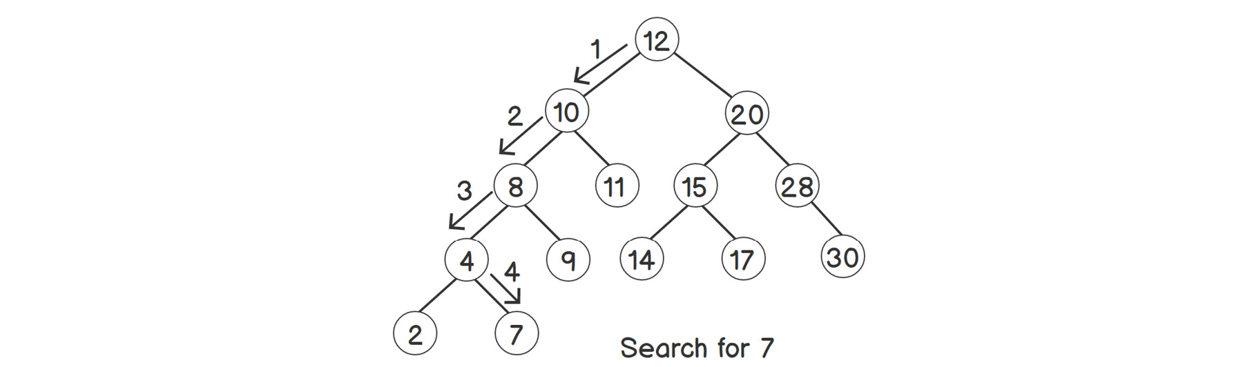
Figure 2.5: Searching for an element in a binary search tree
Let's say that we have to search for 7. As we can see from the steps represented by arrows in the preceding figure, we choose the side after comparing the value with the current node's data. As we've already mentioned, all the nodes on the left will always be less than the current node, and all the nodes on the right will always be greater than the current node.
Thus, we start by comparing the root node with 7. If it is greater than 7, we move to the left subtree, since all the elements there are smaller than the parent node, and vice versa. We compare each child node until we stumble upon 7, or a node less than 7 with no right node. In this case, coming to node 4 leads to our target, 7.
As we can see, we're not traversing the whole tree. Instead, we are reducing our scope by half every time the current node is not the desired one, which we do by choosing either the left or the right side. This works similar to a binary search for linear structures, which we will learn about in Chapter 4, Divide and Conquer.
Inserting a New Element into a BST
Now, let's look at how insertion works. The steps are shown in the following figure:
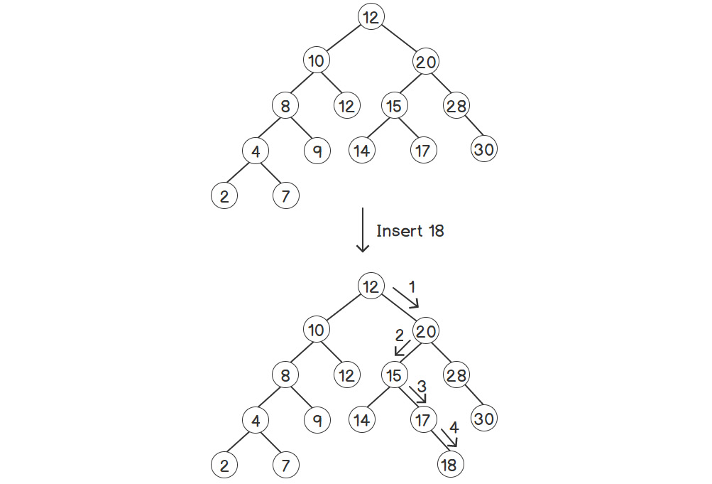
Figure 2.6: Inserting an element into a binary search tree
As you can see, first, we have to find the parent node where we want to insert the new value. Thus, we have to take a similar approach to the one we took for searching; that is, by going in the direction based on comparing each node with our new element, starting with the root node. At the last step, 18 is greater than 17, but 17 doesn't have a right child. Therefore, we insert 18 in that position.
Deleting an Element from a BST
Now, let's look at how deletion works. Consider the following BST:
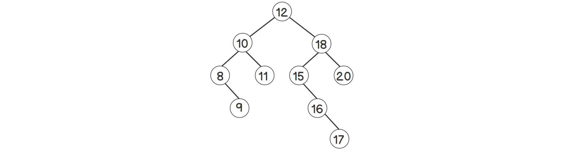
Figure 2.7: Binary search tree rooted at 12
We will delete the root node, 12, in the tree. Let's look at how we can delete any value. It's a bit trickier than insertion since we need to find the replacement of the deleted node so that the properties of the BST remain true.
The first step is to find the node to be deleted. After that, there are three possibilities:
- The node has no children: simply delete the node.
- The node has only one child: point the parent node's corresponding pointer to the only existing child.
- The node has two children: in this case, we replace the current node with its successor.
The successor is the next biggest number after the current node. Or, in other words, the successor is the smallest element among all the elements greater than the current one. Therefore, we'll first go to the right subtree, which contains all the elements greater than the current one, and find the smallest among them. Finding the smallest node means going to the left side of the subtree as much as we can because the left child node is always less than its parent. In the tree shown in figure 2.7, the right subtree of 12 starts at 18. So, we start looking from there, and then try to move down to the left child of 15. But 15 does not have a left child, and the other child, 16, is larger than 15. Hence, 15 should be the successor here.
To replace 12 with 15, first, we will copy the value of the successor at the root while deleting 12, as shown in the following figure:
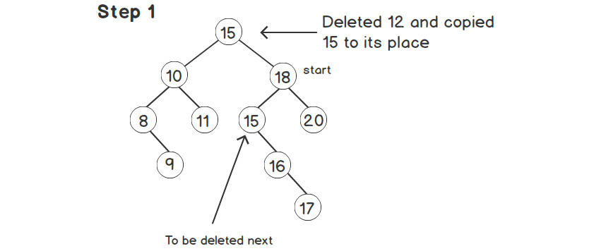
Figure 2.8: Successor copied to the root node
Next, we need to delete the successor, 15, from its old place in the right subtree, as shown in the following figure:
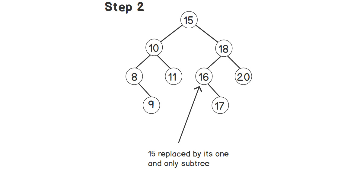
Figure 2.9: Successor deleted from its old place
In the last step, we're deleting node 15. We use the same process for this deletion as well. Since 15 had just one child, we replace the left child of 18 with the child of 15. So, the whole subtree rooted at 16 becomes the left child of 18.
Note
The successor node can only have one child at most. If it had a left child, we would have picked that child and not the current node as the successor.
Time Complexities of Operations on a Tree
Now, let's look at the time complexity of these functions. Theoretically, we can say that we reduce the scope of the search by half each time. Hence, the time that's required to search for the BST with n nodes is T(n) = T(n / 2) + 1. This equation results in a time complexity of T(n) = O(log n).
But there's a catch to this. If we look at the insertion function closely, the order of insertion actually determines the shape of the tree. And it is not necessarily true that we'll always reduce the scope of the search by half, as described by T(n/2) in the previous formula. Therefore, the complexity O(log n) is not always accurate. We'll look at this problem and its solution in more depth in the Balanced Tree section, where we will see how we can calculate time complexity more accurately.
For now, let's implement the operations we just saw in C++.
Exercise 9: Implementing a Binary Search Tree
In this exercise, we will implement the BST shown in figure 2.7 and add a find function to search for elements. We will also try our hand at the insertion and deletion of elements, as explained in the previous subsections. Let's get started:
- First, let's include the required headers:
#include <iostream>
- Now, let's write a node. This will be similar to our previous exercise, except we'll have an integer instead of a string:
struct node
{
int data;
node *left, *right;
};
- Now, let's add a wrapper over the node to provide a clean interface:
struct bst
{
node* root = nullptr;
- Before writing the insertion function, we'll need to write the find function:
node* find(int value)
{
return find_impl(root, value);
}
private:
node* find_impl(node* current, int value)
{
if(!current)
{
std::cout << std::endl;
return NULL;
}
if(current->data == value)
{
std::cout << "Found " << value << std::endl;
return current;
}
if(value < current->data) // Value will be in the left subtree
{
std::cout << "Going left from " << current->data << ", ";
return find_impl(current->left, value);
}
if(value > current->data) // Value will be in the right subtree
{
std::cout << "Going right from " << current->data << ", ";
return find_impl(current->right, value);
}
}
Since this is recursive, we have kept the implementation in a separate function and made it private so as to prevent someone from using it directly.
- Now, let's write an insert function. It will be similar to the find function, but with small tweaks. First, let's find the parent node, which is where we want to insert the new value:
public:
void insert(int value)
{
if(!root)
root = new node{value, NULL, NULL};
else
insert_impl(root, value);
}
private:
void insert_impl(node* current, int value)
{
if(value < current->data)
{
if(!current->left)
current->left = new node{value, NULL, NULL};
else
insert_impl(current->left, value);
}
else
{
if(!current->right)
current->right = new node{value, NULL, NULL};
else
insert_impl(current->right, value);
}
}
As we can see, we are checking whether the value should be inserted in the left or right subtree. If there's nothing on the desired side, we directly insert the node there; otherwise, we call the insert function for that side recursively.
- Now, let's write an inorder traversal function. In-order traversal provides an important advantage when applied to BST, as we will see in the output:
public:
void inorder()
{
inorder_impl(root);
}
private:
void inorder_impl(node* start)
{
if(!start)
return;
inorder_impl(start->left); // Visit the left sub-tree
std::cout << start->data << " "; // Print out the current node
inorder_impl(start->right); // Visit the right sub-tree
}
- Now, let's implement a utility function to get the successor:
public:
node* successor(node* start)
{
auto current = start->right;
while(current && current->left)
current = current->left;
return current;
}
This follows the logic we discussed in the Deleting an Element in BST subsection.
- Now, let's look at the actual implementation of delete. Since deletion requires repointing the parent node, we'll do that by returning the new node every time. We'll hide this complexity by putting a better interface over it. We'll name the interface deleteValue since delete is a reserved keyword, as per the C++ standard:
void deleteValue(int value)
{
root = delete_impl(root, value);
}
private:
node* delete_impl(node* start, int value)
{
if(!start)
return NULL;
if(value < start->data)
start->left = delete_impl(start->left, value);
else if(value > start->data)
start->right = delete_impl(start->right, value);
else
{
if(!start->left) // Either both children are absent or only left child is absent
{
auto tmp = start->right;
delete start;
return tmp;
}
if(!start->right) // Only right child is absent
{
auto tmp = start->left;
delete start;
return tmp;
}
auto succNode = successor(start);
start->data = succNode->data;
// Delete the successor from right subtree, since it will always be in the right subtree
start->right = delete_impl(start->right, succNode->data);
}
return start;
}
};
- Let's write the main function so that we can use the BST:
int main()
{
bst tree;
tree.insert(12);
tree.insert(10);
tree.insert(20);
tree.insert(8);
tree.insert(11);
tree.insert(15);
tree.insert(28);
tree.insert(4);
tree.insert(2);
std::cout << "Inorder: ";
tree.inorder(); // This will print all the elements in ascending order
std::cout << std::endl;
tree.deleteValue(12);
std::cout << "Inorder after deleting 12: ";
tree.inorder(); // This will print all the elements in ascending order
std::cout << std::endl;
if(tree.find(12))
std::cout << "Element 12 is present in the tree" << std::endl;
else
std::cout << "Element 12 is NOT present in the tree" << std::endl;
}
The output upon executing the preceding code should be as follows:
Inorder: 2 4 8 10 11 12 15 20 28
Inorder after deleting 12: 2 4 8 10 11 15 20 28
Going left from 15, Going right from 10, Going right from 11,
Element 12 is NOT present in the tree
Observe the preceding results of in-order traversal for a BST. In-order will visit the left subtree first, then the current node, and then the right subtree, recursively, as shown in the comments in the code snippet. So, as per BST properties, we'll visit all the values smaller than the current one first, then the current one, and after that, we'll visit all the values greater than the current one. And since this happens recursively, we'll get our data sorted in ascending order.
Balanced Tree
Before we understand a balanced tree, let's start with an example of a BST for the following insertion order:
bst tree;
tree.insert(10);
tree.insert(9);
tree.insert(11);
tree.insert(8);
tree.insert(7);
tree.insert(6);
tree.insert(5);
tree.insert(4);
This BST can be visualized with the help of the following figure:
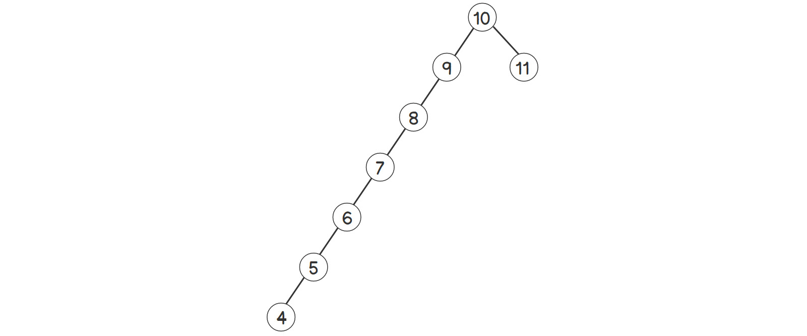
Figure 2.10: Skewed binary search tree
As shown in the preceding figure, almost the whole tree is skewed to the left side. If we call the find function, that is, bst.find(4), the steps will look as follows:
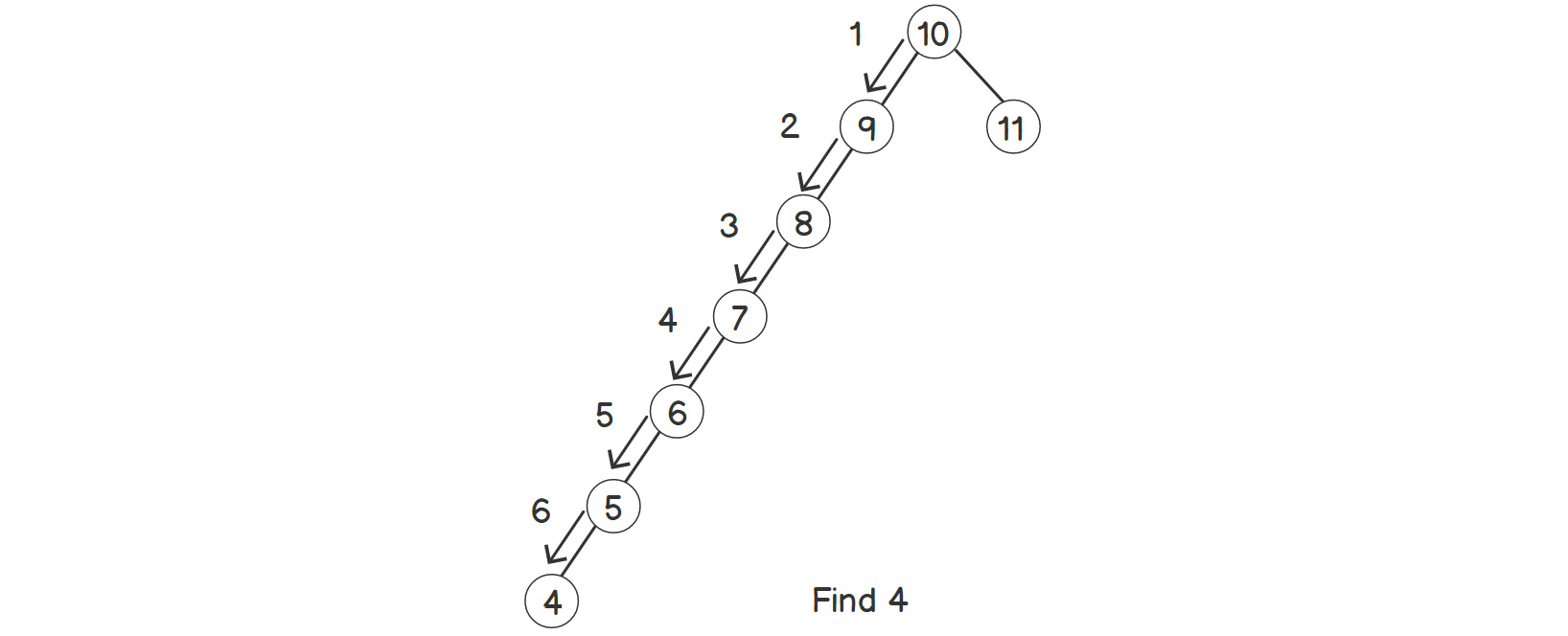
Figure 2.11: Finding an element in a skewed binary search tree
As we can see, the number of steps is almost equal to the number of elements. Now, let's try the same thing again with a different insertion order, as shown here:
bst tree;
tree.insert(7);
tree.insert(5);
tree.insert(9);
tree.insert(4);
tree.insert(6);
tree.insert(10);
tree.insert(11);
tree.insert(8);
The BST and the steps required to find element 4 will now look as follows:
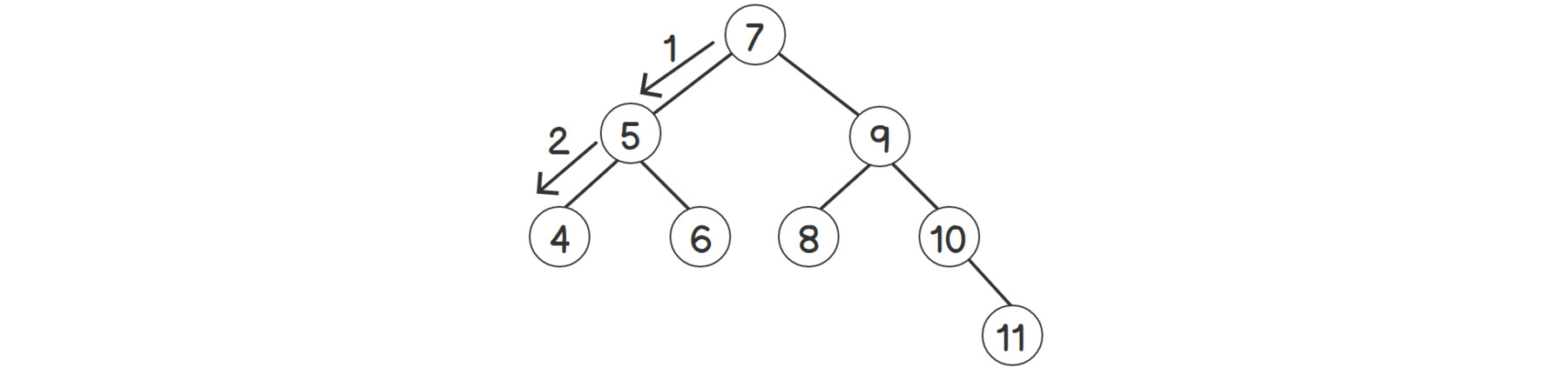
Figure 2.12: Finding an element in a balanced tree
As we can see, the tree is not skewed anymore. Or, in other words, the tree is balanced. The steps to find 4 have been considerably reduced with this configuration. Thus, the time complexity of find is not just dependent on the number of elements, but also on their configuration in the tree. If we look at the steps closely, we are always going one step toward the bottom of the tree while searching for something. And at the end, we end up at the leaf nodes (nodes without any children). Here, we return either the desired node or NULL based on the availability of the element. So, we can say that the number of steps is always less than the maximum number of levels in the BST, also known as the height of the BST. So, the actual time complexity for finding an element is O(height).
In order to optimize the time complexity, we need to optimize the height of the tree. This is also called balancing a tree. The idea is to reorganize the nodes after insertion/deletion to reduce the skewness of the tree. The resultant tree is called a height-balanced BST.
There are various ways in which we can do this and get different types of trees, such as an AVL tree, a Red-Black tree, and so on. The idea behind an AVL tree is to perform some rotations to balance the height of the tree, while still maintaining the BST properties. Consider the example that's shown in the following figure:
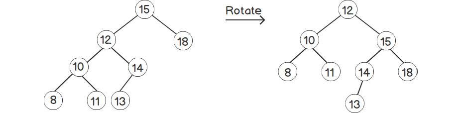
Figure 2.13: Rotating a tree
As we can see, the tree on the right is more balanced compared to the one on the left. Rotation is out of the scope of this book and so we will not venture into the details of this example.
N-ary Tree
Up until now, we've mainly seen binary trees or their variants. For an N-ary tree, each node can have N children. Since N is arbitrary here, we are going to store it in a vector. So, the final structure looks something like this:
struct nTree
{
int data;
std::vector<nTree*> children;
};
As we can see, there can be any number of children for each node. Hence, the whole tree is completely arbitrary. However, just like a plain binary tree, a plain N-ary tree also isn't very useful. Therefore, we have to build a different tree for different kinds of applications, where the hierarchy is of a higher degree than a binary tree. The example shown in figure 2.1, which represents an organization's hierarchy, is an N-ary tree.
In the computer world, there are two really good, well-known implementations of N-ary trees, as follows:
- Filesystem structures in computers: Starting from root (/) in Linux or drives in Windows, we can have any number of files (terminal nodes) and any number of folders inside any folder. We'll look at this in greater detail in Activity 1, Creating a Data Structure for a Filesystem.
- Compilers: Most compilers build an Abstract Syntax Tree (AST) based on syntax defined by the standard that's used for the source code. Compilers generate lower-level code by parsing the AST.
Activity 4: Create a Data Structure for a Filesystem
Create a data structure using an N-ary tree for a filesystem that supports the following operations: go to directory, find file/directory, add file/directory, and list file/directory. Our tree will hold the information and folder hierarchy (path) of all the elements (files and folders) in the filesystem.
Perform the following steps to solve this activity:
- Create an N-ary tree with two data elements in a node – the name of the directory/file and a flag indicating whether it's a directory or a file.
- Add a data member to store the current directory.
- Initialize the tree with a single directory root (/).
- Add the find directory/file function, which takes a single parameter – path. The path can be either absolute (starting with /) or relative.
- Add functions to add a file/directory and list files/directories located at a given path.
- Similarly, add a function to change the current directory.
Note
The solution to this activity can be found on page 490.
We've printed directories with d in front to distinguish them from files, which are printed with a "–" (hyphen) in front. You can experiment by creating more directories and files with absolute or relative paths.
So far, we haven't supported certain Linux conventions, such as addressing any directory with a single dot and addressing a parent directory with double dots. This can be done by extending our node to also hold a pointer to its parent node. This way, we can traverse in both directions very easily. There are various other extensions possible, such as the addition of symlinks, as well as globing operators to expand the names of the various files/directories using "*". This exercise provides us with a base so that we can build something on our own based on our requirements.
Heaps
In the previous chapter, we had a brief look at heaps and how C++ provides heaps via STL. In this chapter, we'll take a deeper look at heaps. Just to recap, the following are the intended time complexities:
- O(1): Immediate access to the max element
- O(log n): Insertion of any element
- O(log n): Deletion of the max element
To achieve O(log n) insertion/deletion, we'll use a tree to store data. But in this case, we'll 'use a complete tree. A complete tree is defined as a tree where nodes at all the levels except the last one have two children, and the last level has as many of the elements on the left side as possible. For example, consider the two trees shown in the following figure:
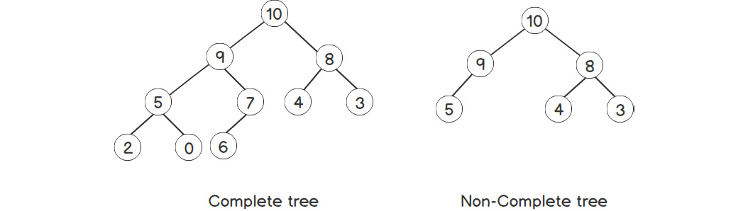
Figure 2.14: Complete versus non-complete tree
Thus, a complete tree can be constructed by inserting elements in the last level, as long as there's enough space there. If not, we will insert them at the leftmost position on the new level. This gives us a very good opportunity to store this tree using an array, level by level. So, the root of the tree will be the first element of the array/vector, followed by its left child and then the right child, and so on. Unlike other trees, this is a very efficient memory structure because there is no extra memory required to store pointers. To go from a parent to its child node, we can easily use the index of the array. If the parent is the ith node, its children will always be 2*i + 1 and 2*i + 2 indices. And similarly, we can get the parent node for the ith child node by using (i – 1) / 2. We can also confirm this from the preceding figure.
Now, let's have a look at the invariants (or conditions) we need to maintain upon every insertion/deletion. The first requirement is instant access to the max element. For that, we need to fix its position so that it is accessible immediately every time. We'll always keep our max element at the top – the root position. Now, to maintain this, we also need to maintain another invariant – the parent node must be greater than both of its children. Such a heap is also known as a max heap.
As you can probably guess, the properties that are required for fast access to the maximum element can be easily inverted for fast access to the minimum element. All we need to do is invert our comparison function while performing heap operations. This kind of heap is known as a min heap.
Heap Operations
In this section, we will see how we can perform different operations on a heap.
Inserting an Element into a Heap
As the first step of insertion, we will preserve the most important invariant, which provides us with a way to represent this structure as an array – a complete tree. This can easily be done by inserting the new element at the end since it will represent the element in the last level, right after all the existing elements, or as the first element in a new level if the current last level is full.
Now, we need to preserve the other invariant – all the nodes must have a value greater than both of their children, if available. Assuming that our current tree is already following this invariant, after the insertion of the new element in the last position, the only element where the invariant may fail would be the last element. To resolve this, we swap the element with its parent if the parent is smaller than the element. Even if the parent already has another element, it will be smaller than the new element (new element > parent > child).
Thus, the subtree that's created by considering the new element as the root satisfies all the invariants. However, the new element may still be greater than its new parent. Therefore, we need to keep on swapping the nodes until the invariant is satisfied for the whole tree. Since the height of a complete tree is O(log n) at most, the entire operation will take a maximum of O(log n) time. The following figure illustrates the operation of inserting elements into a tree:
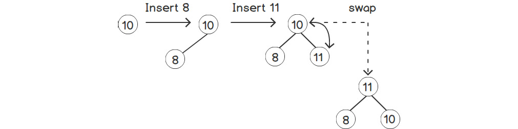
Figure 2.15: Inserting an element into a heap with one node
As shown in the preceding figure, after inserting 11, the tree doesn't have the heap property anymore. Therefore, we'll swap 10 and 11 to make it a heap again. This concept is clearer with the following example, which has more levels:
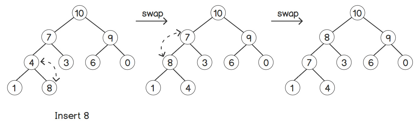
Figure 2.16: Inserting an element into a heap with several nodes
Deleting an Element from a Heap
The first thing to notice is that we can only delete the max element. We can't directly touch any other element. The max element is always present at the root. Hence, we'll remove the root element. But we also need to decide who'll take its position. For that, we first need to swap the root with the last element, and then remove the last element.That way, our root will be deleted, but it will break the invariant of having each parent node greater than its children. To resolve this, we'll compare the root with its two children and swap it with the greater one. Now, the invariant is broken at one of the subtrees. We continue the swapping process recursively throughout the subtree. That way, the breaking point of the invariant is bubbled down the tree. Just like insertion, we follow this until we meet the invariant. The maximum number of steps required will be equal to the height of the tree, which is O(log n). The following figure illustrates this process:
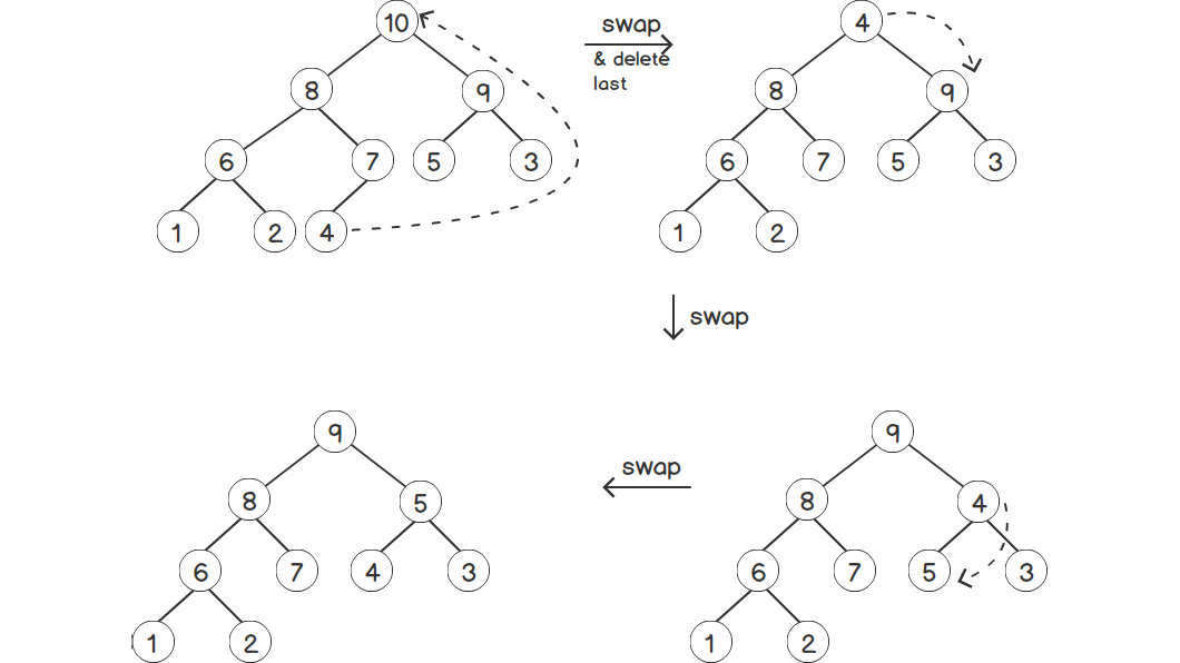
Figure 2.17: Deleting an element in a heap
Initialization of a Heap
Now, let's look at one of the most important steps – the initialization of a heap. Unlike vectors, lists, deques, and so on, a heap is not simple to initialize because we need to maintain the invariants of the heap. One easy solution would be to insert all the elements starting from an empty heap, one by one. But the time required for this would be O(n * log(n)), which is not efficient.
However, there's a heapification algorithm that can do this in O(n) time. The idea behind this is very simple: we keep on updating the tree to match the heap properties for smaller subtrees in a bottom-up manner. For starters, the last level already has the properties of a heap. Followed by that, we go level by level toward the root, making each subtree follow the heap properties one by one. This process only has a time complexity of O(n). And fortunately, the C++ standard already provides a function for this called std::make_heap, which can take any array or vector iterators and convert them into a heap.
Exercise 10: Streaming Median
In this exercise, we'll solve an interesting problem that frequently occurs in data analysis-related applications, including machine learning. Imagine that some source is giving us data one element at a time continuously (a stream of data). We need to find the median of the elements that have been received up until now after receiving each and every element. One simple way of doing this would be to sort the data every time a new element comes in and return the middle element. But this would have an O(n log n) time complexity because of sorting. Depending on the rate of incoming elements, this can be very resource-intensive. However, we'll optimize this with the help of heaps. Let's get started:
- Let's include the required headers first:
#include <queue>
#include <vector>
- Now, let's write a container to store the data we've received up until now. We'll store the data among two heaps – one min heap and one max heap. We'll store the smaller, first half of the elements in a max heap, and the larger, or the other half, in a min heap. So, at any point, the median can be calculated using only the top elements of the heaps, which are easily accessible:
struct median
{
std::priority_queue<int> maxHeap;
std::priority_queue<int, std::vector<int>, std::greater<int>> minHeap;
- Now, let's write an insert function so that we can insert the newly arrived data:
void insert(int data)
{
// First element
if(maxHeap.size() == 0)
{
maxHeap.push(data);
return;
}
if(maxHeap.size() == minHeap.size())
{
if(data <= get())
maxHeap.push(data);
else
minHeap.push(data);
return;
}
if(maxHeap.size() < minHeap.size())
{
if(data > get())
{
maxHeap.push(minHeap.top());
minHeap.pop();
minHeap.push(data);
}
else
maxHeap.push(data);
return;
}
if(data < get())
{
minHeap.push(maxHeap.top());
maxHeap.pop();
maxHeap.push(data);
}
else
minHeap.push(data);
}
- Now, let's write a get function so that we can get the median from the containers:
double get()
{
if(maxHeap.size() == minHeap.size())
return (maxHeap.top() + minHeap.top()) / 2.0;
if(maxHeap.size() < minHeap.size())
return minHeap.top();
return maxHeap.top();
}
};
- Now, let's write a main function so that we can use this class:
int main()
{
median med;
med.insert(1);
std::cout << "Median after insert 1: " << med.get() << std::endl;
med.insert(5);
std::cout << "Median after insert 5: " << med.get() << std::endl;
med.insert(2);
std::cout << "Median after insert 2: " << med.get() << std::endl;
med.insert(10);
std::cout << "Median after insert 10: " << med.get() << std::endl;
med.insert(40);
std::cout << "Median after insert 40: " << med.get() << std::endl;
return 0;
}
The output of the preceding program is as follows:
Median after insert 1: 1
Median after insert 5: 3
Median after insert 2: 2
Median after insert 10: 3.5
Median after insert 40: 5
This way, we only need to insert any newly arriving elements, which only has a time complexity of O(log n), compared to the time complexity of O(n log n) if we were to sort the elements with each new element.
Activity 5: K-Way Merge Using Heaps
Consider a biomedical application related to genetics being used for processing large datasets. It requires ranks of DNA in a sorted manner to calculate similarity. But since the dataset is huge, it can't fit on a single machine. Therefore, it processes and stores data in a distributed cluster, and each node has a set of sorted values. The main processing engine requires all of the data to be in a sorted fashion and in a single stream. So, basically, we need to merge multiple sorted arrays into a single sorted array. Simulate this situation with the help of vectors.
Perform the following steps to solve this activity:
- The smallest number will be present in the first element of all the lists since all the lists have already been sorted individually. To get that minimum faster, we'll build a heap of those elements.
- After getting the minimum element from the heap, we need to remove it and replace it with the next element from the same list it belongs to.
- The heap node must contain information about the list so that it can find the next number from that list.
Note
The solution to this activity can be found on page 495.
Now, let's calculate the time complexity of the preceding algorithm. If there are k lists available, our heap size will be k, and all of our heap operations will be O(log k). Building heap will be O(k log k). After that, we'll have to perform a heap operation for each element in the result. The total elements are n × k. Therefore, the total complexity will be O(nk log k).
The wonderful thing about this algorithm is that, considering the real-life scenario we described earlier, it doesn't actually need to store all the n × k elements at the same time; it only needs to store k elements at any point in time, where k is the number of lists or nodes in the cluster. Due to this, the value of k will never be too large. With the help of a heap, we can generate one number at a time and either process the number immediately or stream it elsewhere for processing without actually storing it.
Graphs
Although a tree is a pretty good way to represent hierarchical data, we can't represent circular or cyclic dependencies in a tree because we always have a single and unique path to go from one node to another. However, there are more complex scenarios that have a cyclic structure inherently. For example, consider a road network. There can be multiple ways to go from one place (places can be represented as nodes) to another. Such a set of scenarios can be better represented using graphs.
Unlike a tree, a graph has to store data for the nodes, as well as for the edges between the nodes. For example, in any road network, for each node (place), we have to store the information about which other nodes (places) it connects to. This way, we can form a graph with all the required nodes and edges. This is called an unweighted graph. We can add weights, or more information, to each of the edges. For our road network example, we can add the distance of each edge (path) from one node (place) to another. This representation, called a weighted graph, has all the information about a road network that's required to solve problems such as finding the path that has the minimum distance between one place and another.
There are two types of graphs – undirected and directed. An undirected graph indicates that the edges are bidirectional. Bidirectional indicates a bilateral or commutative property. For the road network example, a bidirectional edge between points A and B implies that we can go from A to B, as well as from B to A. But let's say we have some roads with a one-way restriction – we need to use a directed graph to represent that. In a direct graph, whenever we need to indicate that we can go in either direction, we use two edges – from point A to B, and B to A. We'll mainly focus on bidirectional graphs, but the things we'll learn here about structure and traversing methods hold true for directed graphs as well. The only change will be how we add edges to the graph.
Since a graph can have cyclic edges and more than one way to go from one node to another, we need to identify each node uniquely. For that, we can assign an identifier to each node. To represent the graph's data, we don't really need to build a node-like structure programmatically, as we did in trees. In fact, we can store the whole graph by combining std containers.
Representing a Graph as an Adjacency Matrix
Here is one of the simplest ways to understand a graph – consider a set of nodes, where any node can connect to any other node among the set directly. This means that we can represent this using a 2D array that's N × N in size for a graph with N nodes. The value in each cell will indicate the weight of the edge between the corresponding nodes based on the indices of the cell. So, data[1][2] will indicate the weight of the edge between node 1 and node 2. This method is known as an adjacency matrix. We can indicate the absence of an edge using a weight of -1.
Consider the weighted graph shown in the following figure, which represents an aviation network between a few major international cities, with hypothetical distances:
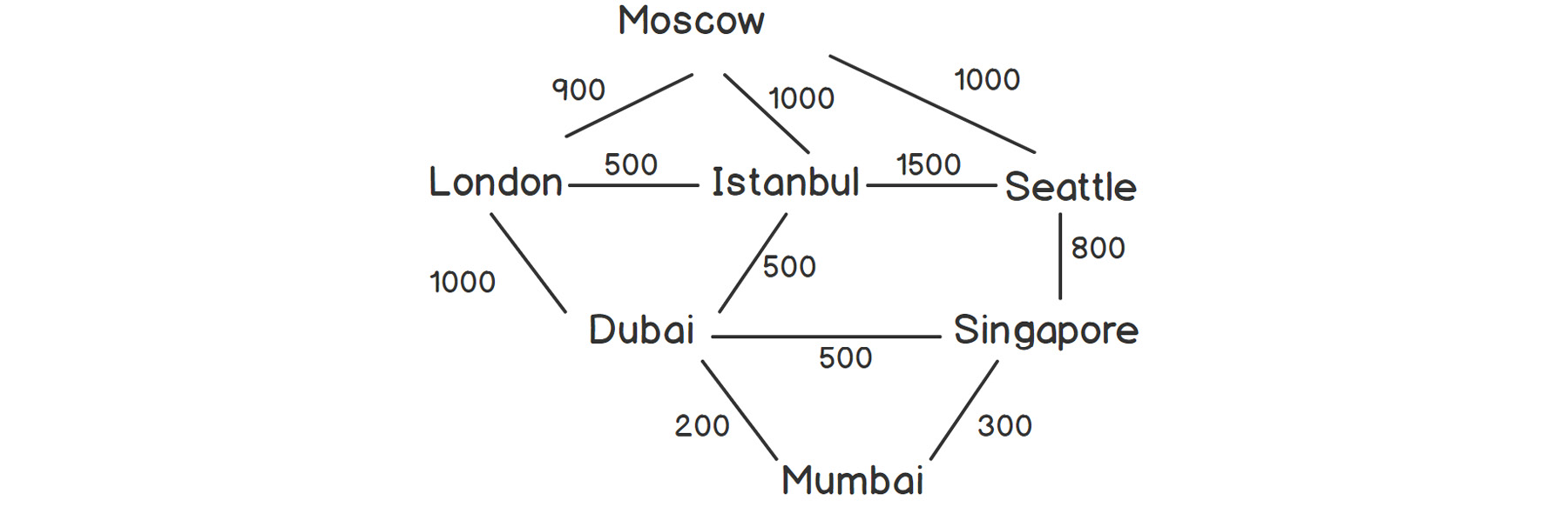
Figure 2.18: Aviation network between some cities
As shown in the preceding figure, we can go from London to Dubai via Istanbul or directly. There are multiple ways to go from one place to another, which was not the case with trees. Also, we can traverse from one node to another and come back to the original node via some different edges, which was also not possible in a tree.
Let's implement the matrix representation method for the graph shown in the preceding figure.
Exercise 11: Implementing a Graph and Representing it as an Adjacency Matrix
In this exercise, we will implement a graph representing the network of cities shown in the preceding figure, and demonstrate how it can be stored as an adjacency matrix. Let's get started:
- First, let's include the required headers:
#include <iostream>
#include <vector>
- Now, let's add an enum class so that we can store the names of the cities:
enum class city: int
{
LONDON,
MOSCOW,
ISTANBUL,
DUBAI,
MUMBAI,
SEATTLE,
SINGAPORE
};
- Let's also add a << operator for the city enum:
std::ostream& operator<<(std::ostream& os, const city c)
{
switch(c)
{
case city::LONDON:
os << "LONDON";
return os;
case city::MOSCOW:
os << "MOSCOW";
return os;
case city::ISTANBUL:
os << "ISTANBUL";
return os;
case city::DUBAI:
os << "DUBAI";
return os;
case city::MUMBAI:
os << "MUMBAI";
return os;
case city::SEATTLE:
os << "SEATTLE";
return os;
case city::SINGAPORE:
os << "SINGAPORE";
return os;
default:
return os;
}
}
- Let's write the struct graph, which will encapsulate our data:
struct graph
{
std::vector<std::vector<int>> data;
- Now, let's add a constructor that will create an empty graph (a graph without any edges) with a given number of nodes:
graph(int n)
{
data.reserve(n);
std::vector<int> row(n);
std::fill(row.begin(), row.end(), -1);
for(int i = 0; i < n; i++)
{
data.push_back(row);
}
}
- Now, let's add the most important function – addEdge. It will take three parameters – the two cities to be connected and the weight (distance) of the edge:
void addEdge(const city c1, const city c2, int dis)
{
std::cout << "ADD: " << c1 << "-" << c2 << "=" << dis << std::endl;
auto n1 = static_cast<int>(c1);
auto n2 = static_cast<int>(c2);
data[n1][n2] = dis;
data[n2][n1] = dis;
}
- Now, let's add a function so that we can remove an edge from the graph:
void removeEdge(const city c1, const city c2)
{
std::cout << "REMOVE: " << c1 << "-" << c2 << std::endl;
auto n1 = static_cast<int>(c1);
auto n2 = static_cast<int>(c2);
data[n1][n2] = -1;
data[n2][n1] = -1;
}
};
- Now, let's write the main function so that we can use these functions:
int main()
{
graph g(7);
g.addEdge(city::LONDON, city::MOSCOW, 900);
g.addEdge(city::LONDON, city::ISTANBUL, 500);
g.addEdge(city::LONDON, city::DUBAI, 1000);
g.addEdge(city::ISTANBUL, city::MOSCOW, 1000);
g.addEdge(city::ISTANBUL, city::DUBAI, 500);
g.addEdge(city::DUBAI, city::MUMBAI, 200);
g.addEdge(city::ISTANBUL, city::SEATTLE, 1500);
g.addEdge(city::DUBAI, city::SINGAPORE, 500);
g.addEdge(city::MOSCOW, city::SEATTLE, 1000);
g.addEdge(city::MUMBAI, city::SINGAPORE, 300);
g.addEdge(city::SEATTLE, city::SINGAPORE, 700);
g.addEdge(city::SEATTLE, city::LONDON, 1800);
g.removeEdge(city::SEATTLE, city::LONDON);
return 0;
}
- Upon executing this program, we should get the following output:
ADD: LONDON-MOSCOW=900
ADD: LONDON-ISTANBUL=500
ADD: LONDON-DUBAI=1000
ADD: ISTANBUL-MOSCOW=1000
ADD: ISTANBUL-DUBAI=500
ADD: DUBAI-MUMBAI=200
ADD: ISTANBUL-SEATTLE=1500
ADD: DUBAI-SINGAPORE=500
ADD: MOSCOW-SEATTLE=1000
ADD: MUMBAI-SINGAPORE=300
ADD: SEATTLE-SINGAPORE=700
ADD: SEATTLE-LONDON=1800
REMOVE: SEATTLE-LONDON
As we can see, we are storing the data in a vector of a vector, with both dimensions equal to the number of nodes. Hence, the total space required for this representation is proportional to V2, where V is the number of nodes.
Representing a Graph as an Adjacency List
A major problem with a matrix representation of a graph is that the amount of memory required is directly proportional to the number of nodes squared. As you might imagine, this adds up quickly with the number of nodes. Let's see how we can improve this so that we use less memory.
In any graph, we'll have a fixed number of nodes, and each node will have a fixed maximum number of connected nodes, which is equal to the total nodes. In a matrix, we have to store all the edges for all the nodes, even if two nodes are not directly connected to each other. Instead, we'll only store the IDs of the nodes in each row, indicating which nodes are directly connected to the current one. This representation is also called an adjacency list.
Let's see how the implementation differs compared to the previous exercise.
Exercise 12: Implementing a Graph and Representing it as an Adjacency List
In this exercise, we will implement a graph representing the network of cities shown in figure 2.18, and demonstrate how it can be stored as an adjacency list. Let's get started:
- We'll implement an adjacency list representation in this exercise. Let's start with headers, as usual:
#include <iostream>
#include <vector>
#include <algorithm>
- Now, let's add an enum class so that we can store the names of the cities:
enum class city: int
{
MOSCOW,
LONDON,
ISTANBUL,
SEATTLE,
DUBAI,
MUMBAI,
SINGAPORE
};
- Let's also add the << operator for the city enum:
std::ostream& operator<<(std::ostream& os, const city c)
{
switch(c)
{
case city::MOSCOW:
os << "MOSCOW";
return os;
case city::LONDON:
os << "LONDON";
return os;
case city::ISTANBUL:
os << "ISTANBUL";
return os;
case city::SEATTLE:
os << "SEATTLE";
return os;
case city::DUBAI:
os << "DUBAI";
return os;
case city::MUMBAI:
os << "MUMBAI";
return os;
case city::SINGAPORE:
os << "SINGAPORE";
return os;
default:
return os;
}
}
- Let's write the struct graph, which will encapsulate our data:
struct graph
{
std::vector<std::vector<std::pair<int, int>>> data;
- Let's see how our constructor defers from a matrix representation:
graph(int n)
{
data = std::vector<std::vector<std::pair<int, int>>>(n, std::vector<std::pair<int, int>>());
}
As we can see, we are initializing the data with a 2D vector, but all the rows are initially empty because there are no edges present at the start.
- Let's implement the addEdge function for this:
void addEdge(const city c1, const city c2, int dis)
{
std::cout << "ADD: " << c1 << "-" << c2 << "=" << dis << std::endl;
auto n1 = static_cast<int>(c1);
auto n2 = static_cast<int>(c2);
data[n1].push_back({n2, dis});
data[n2].push_back({n1, dis});
}
- Now, let's write removeEdge so that we can remove an edge from the graph:
void removeEdge(const city c1, const city c2)
{
std::cout << "REMOVE: " << c1 << "-" << c2 << std::endl;
auto n1 = static_cast<int>(c1);
auto n2 = static_cast<int>(c2);
std::remove_if(data[n1].begin(), data[n1].end(), [n2](const auto& pair)
{
return pair.first == n2;
});
std::remove_if(data[n2].begin(), data[n2].end(), [n1](const auto& pair)
{
return pair.first == n1;
});
}
};
- Now, let's write the main function so that we can use these functions:
int main()
{
graph g(7);
g.addEdge(city::LONDON, city::MOSCOW, 900);
g.addEdge(city::LONDON, city::ISTANBUL, 500);
g.addEdge(city::LONDON, city::DUBAI, 1000);
g.addEdge(city::ISTANBUL, city::MOSCOW, 1000);
g.addEdge(city::ISTANBUL, city::DUBAI, 500);
g.addEdge(city::DUBAI, city::MUMBAI, 200);
g.addEdge(city::ISTANBUL, city::SEATTLE, 1500);
g.addEdge(city::DUBAI, city::SINGAPORE, 500);
g.addEdge(city::MOSCOW, city::SEATTLE, 1000);
g.addEdge(city::MUMBAI, city::SINGAPORE, 300);
g.addEdge(city::SEATTLE, city::SINGAPORE, 700);
g.addEdge(city::SEATTLE, city::LONDON, 1800);
g.removeEdge(city::SEATTLE, city::LONDON);
return 0;
}
Upon executing this program, we should get the following output:
ADD: LONDON-MOSCOW=900
ADD: LONDON-ISTANBUL=500
ADD: LONDON-DUBAI=1000
ADD: ISTANBUL-MOSCOW=1000
ADD: ISTANBUL-DUBAI=500
ADD: DUBAI-MUMBAI=200
ADD: ISTANBUL-SEATTLE=1500
ADD: DUBAI-SINGAPORE=500
ADD: MOSCOW-SEATTLE=1000
ADD: MUMBAI-SINGAPORE=300
ADD: SEATTLE-SINGAPORE=700
ADD: SEATTLE-LONDON=1800
REMOVE: SEATTLE-LONDON
Since we are storing a list of adjacent nodes for each node, this method is called an adjacency list. This method also uses a vector of a vector to store the data, just like the former method. But the dimension of the inner vector is not equal to the number of nodes; instead, it depends on the number of edges. For each edge in the graph, we'll have two entries, as per our addEdge function. The memory that's required for this type of representation would be proportional to E, where E is the number of edges.
Up until now, we've only seen how to build a graph. We need to traverse a graph to be able to perform any operations while using it. There are two widely used methods available – Breadth-First Search (BFS) and Depth-First Search (DFS), both of which we'll look at in Chapter 6, Graph Algorithms I.
Summary
In this chapter, we looked at a more advanced class of problems compared to the previous chapter, which helped us to describe a wider range of real-world scenarios. We looked at and implemented two major data structures – trees and graphs. We also looked at various types of trees that we can use in different situations. Then, we looked at different ways of representing data programmatically for these structures. With the help of this chapter, you should be able to apply these techniques to solve real-world problems of similar kinds.
Now that we've looked at linear and non-linear data structures, in the next chapter, we'll look at a very specific but widely used concept called lookup, where the goal is to store values in a container so that searching is super fast. We will also look at the fundamental idea behind hashing and how can we implement such a container.