Chapter 4 Parallel Programming in CUDA C
In the previous chapter, we saw how simple it can be to write code that executes on the GPU. We have even gone so far as to learn how to add two numbers together, albeit just the numbers 2 and 7. Admittedly, that example was not immensely impressive, nor was it incredibly interesting. But we hope you are convinced that it is easy to get started with CUDA C and you’re excited to learn more. Much of the promise of GPU computing lies in exploiting the massively parallel structure of many problems. In this vein, we intend to spend this chapter examining how to execute parallel code on the GPU using CUDA C.
4.1 Chapter Objectives
Through the course of this chapter, you will accomplish the following:
• You will learn one of the fundamental ways CUDA exposes its parallelism.
• You will write your first parallel code with CUDA C.
4.2 CUDA Parallel Programming
Previously, we saw how easy it was to get a standard C function to start running on a device. By adding the __global__ qualifier to the function and by calling it using a special angle bracket syntax, we executed the function on our GPU. Although this was extremely simple, it was also extremely inefficient because NVIDIA’s hardware engineering minions have optimized their graphics processors to perform hundreds of computations in parallel. However, thus far we have only ever launched a kernel that runs serially on the GPU. In this chapter, we see how straightforward it is to launch a device kernel that performs its computations in parallel.
4.2.1 Summing Vectors
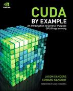
We will contrive a simple example to illustrate threads and how we use them to code with CUDA C. Imagine having two lists of numbers where we want to sum corresponding elements of each list and store the result in a third list. Figure 4.1 shows this process. If you have any background in linear algebra, you will recognize this operation as summing two vectors.
Figure 4.1 Summing two vectors
CPU Vector Sums
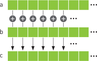
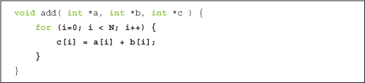
First we’ll look at one way this addition can be accomplished with traditional C code:
Most of this example bears almost no explanation, but we will briefly look at the add() function to explain why we overly complicated it.
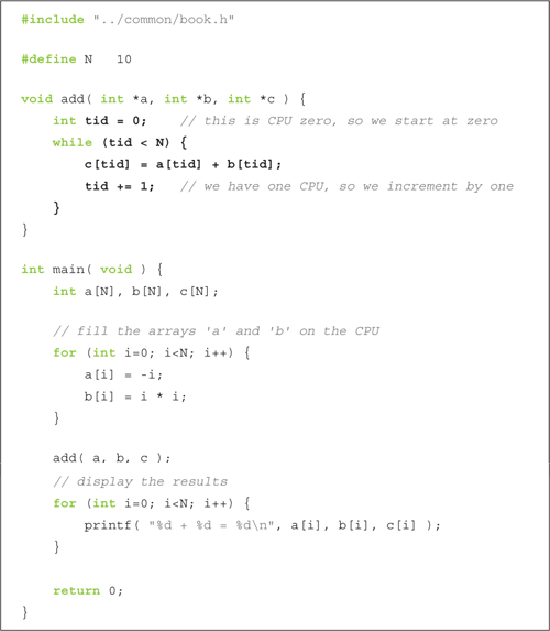
We compute the sum within a while loop where the index tid ranges from 0 to N-1. We add corresponding elements of a[] and b[], placing the result in the corresponding element of c[]. One would typically code this in a slightly simpler manner, like so:
Our slightly more convoluted method was intended to suggest a potential way to parallelize the code on a system with multiple CPUs or CPU cores. For example, with a dual-core processor, one could change the increment to 2 and have one core initialize the loop with tid = 0 and another with tid = 1. The first core would add the even-indexed elements, and the second core would add the odd-indexed elements. This amounts to executing the following code on each of the two CPU cores:
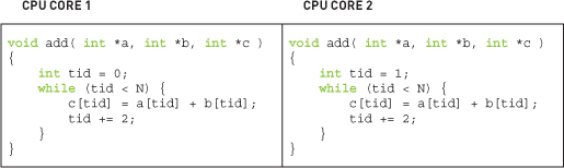
Of course, doing this on a CPU would require considerably more code than we have included in this example. You would need to provide a reasonable amount of infrastructure to create the worker threads that execute the function add() as well as make the assumption that each thread would execute in parallel, a scheduling assumption that is unfortunately not always true.
GPU Vector Sums
We can accomplish the same addition very similarly on a GPU by writing add() as a device function. This should look similar to code you saw in the previous chapter. But before we look at the device code, we present main(). Although the GPU implementation of main() is different from the corresponding CPU version, nothing here should look new:
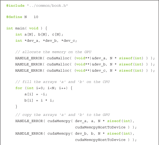
You will notice some common patterns that we employ again:
• We allocate three arrays on the device using calls to cudaMalloc(): two arrays, dev_a and dev_b, to hold inputs, and one array, dev_c, to hold the result.
• Because we are environmentally conscientious coders, we clean up after ourselves with cudaFree().
• Using cudaMemcpy(), we copy the input data to the device with the parameter cudaMemcpyHostToDevice and copy the result data back to the host with cudaMemcpyDeviceToHost.
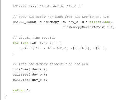
• We execute the device code in add() from the host code in main() using the triple angle bracket syntax.
As an aside, you may be wondering why we fill the input arrays on the CPU. There is no reason in particular why we need to do this. In fact, the performance of this step would be faster if we filled the arrays on the GPU. But we intend to show how a particular operation, namely, the addition of two vectors, can be implemented on a graphics processor. As a result, we ask you to imagine that this is but one step of a larger application where the input arrays a[] and b[] have been generated by some other algorithm or loaded from the hard drive by the user. In summary, it will suffice to pretend that this data appeared out of nowhere and now we need to do something with it.
Moving on, our add() routine looks similar to its corresponding CPU implementation:
Again we see a common pattern with the function add():
• We have written a function called add() that executes on the device. We accomplished this by taking C code and adding a __global__ qualifier to the function name.
So far, there is nothing new in this example except it can do more than add 2 and 7. However, there are two noteworthy components of this example: The parameters within the triple angle brackets and the code contained in the kernel itself both introduce new concepts.
Up to this point, we have always seen kernels launched in the following form:
kernel<<<1,1>>>( param1, param2, . . . );
But in this example we are launching with a number in the angle brackets that is not 1:
add<<<N,1>>>( dev _ a, dev _ b, dev _ c );
What gives?
Recall that we left those two numbers in the angle brackets unexplained; we stated vaguely that they were parameters to the runtime that describe how to launch the kernel. Well, the first number in those parameters represents the number of parallel blocks in which we would like the device to execute our kernel. In this case, we’re passing the value N for this parameter.
For example, if we launch with kernel<<<2,1>>>(), you can think of the runtime creating two copies of the kernel and running them in parallel. We call each of these parallel invocations a block. With kernel<<<256,1>>>(), you would get 256 blocks running on the GPU. Parallel programming has never been easier.
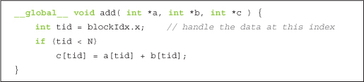
But this raises an excellent question: The GPU runs N copies of our kernel code, but how can we tell from within the code which block is currently running? This question brings us to the second new feature of the example, the kernel code itself. Specifically, it brings us to the variable blockIdx.x:
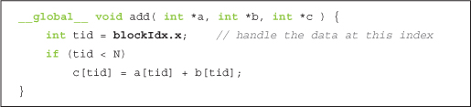
At first glance, it looks like this variable should cause a syntax error at compile time since we use it to assign the value of tid, but we have never defined it. However, there is no need to define the variable blockIdx; this is one of the built-in variables that the CUDA runtime defines for us. Furthermore, we use this variable for exactly what it sounds like it means. It contains the value of the block index for whichever block is currently running the device code.
Why, you may then ask, is it not just blockIdx? Why blockIdx.x? As it turns out, CUDA C allows you to define a group of blocks in two dimensions. For problems with two-dimensional domains, such as matrix math or image processing, it is often convenient to use two-dimensional indexing to avoid annoying translations from linear to rectangular indices. Don’t worry if you aren’t familiar with these problem types; just know that using two-dimensional indexing can sometimes be more convenient than one-dimensional indexing. But you never have to use it. We won’t be offended.
When we launched the kernel, we specified N as the number of parallel blocks. We call the collection of parallel blocks a grid. This specifies to the runtime system that we want a one-dimensional grid of N blocks (scalar values are interpreted as one-dimensional). These threads will have varying values for blockIdx.x, the first taking value 0 and the last taking value N-1. So, imagine four blocks, all running through the same copy of the device code but having different values for the variable blockIdx.x. This is what the actual code being executed in each of the four parallel blocks looks like after the runtime substitutes the appropriate block index for blockIdx.x:
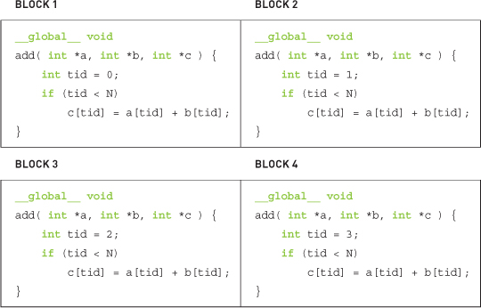
If you recall the CPU-based example with which we began, you will recall that we needed to walk through indices from 0 to N-1 in order to sum the two vectors. Since the runtime system is already launching a kernel where each block will have one of these indices, nearly all of this work has already been done for us. Because we’re something of a lazy lot, this is a good thing. It affords us more time to blog, probably about how lazy we are.
The last remaining question to be answered is, why do we check whether tid is less than N? It should always be less than N, since we’ve specifically launched our kernel such that this assumption holds. But our desire to be lazy also makes us paranoid about someone breaking an assumption we’ve made in our code. Breaking code assumptions means broken code. This means bug reports, late nights tracking down bad behavior, and generally lots of activities that stand between us and our blog. If we didn’t check that tid is less than N and subsequently fetched memory that wasn’t ours, this would be bad. In fact, it could possibly kill the execution of your kernel, since GPUs have sophisticated memory management units that kill processes that seem to be violating memory rules.
If you encounter problems like the ones just mentioned, one of the HANDLE_ERROR() macros that we’ve sprinkled so liberally throughout the code will detect and alert you to the situation. As with traditional C programming, the lesson here is that functions return error codes for a reason. Although it is always tempting to ignore these error codes, we would love to save you the hours of pain through which we have suffered by urging that you check the results of every operation that can fail. As is often the case, the presence of these errors will not prevent you from continuing the execution of your application, but they will most certainly cause all manner of unpredictable and unsavory side effects downstream.
At this point, you’re running code in parallel on the GPU. Perhaps you had heard this was tricky or that you had to understand computer graphics to do general-purpose programming on a graphics processor. We hope you are starting to see how CUDA C makes it much easier to get started writing parallel code on a GPU. We used the example only to sum vectors of length 10. If you would like to see how easy it is to generate a massively parallel application, try changing the 10 in the line #define N 10 to 10000 or 50000 to launch tens of thousands of parallel blocks. Be warned, though: No dimension of your launch of blocks may exceed 65,535. This is simply a hardware-imposed limit, so you will start to see failures if you attempt launches with more blocks than this. In the next chapter, we will see how to work within this limitation.
4.2.2 A Fun Example
We don’t mean to imply that adding vectors is anything less than fun, but the following example will satisfy those looking for some flashy examples of parallel CUDA C.
The following example will demonstrate code to draw slices of the Julia Set. For the uninitiated, the Julia Set is the boundary of a certain class of functions over complex numbers. Undoubtedly, this sounds even less fun than vector addition and matrix multiplication. However, for almost all values of the functions’ parameters, this boundary forms a fractal, one of the most interesting and beautiful curiosities of mathematics.
The calculations involved in generating such a set are quite simple. At its heart, the Julia Set evaluates a simple iterative equation for points in the complex plane. A point is not in the set if the process of iterating the equation diverges for that point. That is, if the sequence of values produced by iterating the equation grows toward infinity, a point is considered outside the set. Conversely, if the values taken by the equation remain bounded, the point is in the set.
Computationally, the iterative equation in question is remarkably simple, as shown in Equation 4.1.
![]()
Computing an iteration of Equation 4.1 would therefore involve squaring the current value and adding a constant to get the next value of the equation.
CPU Julia Set
We will examine a source listing now that will compute and visualize the Julia Set. Since this is a more complicated program than we have studied so far, we will split it into pieces here. Later in the chapter, you will see the entire source listing.
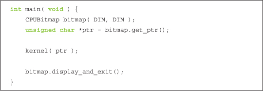
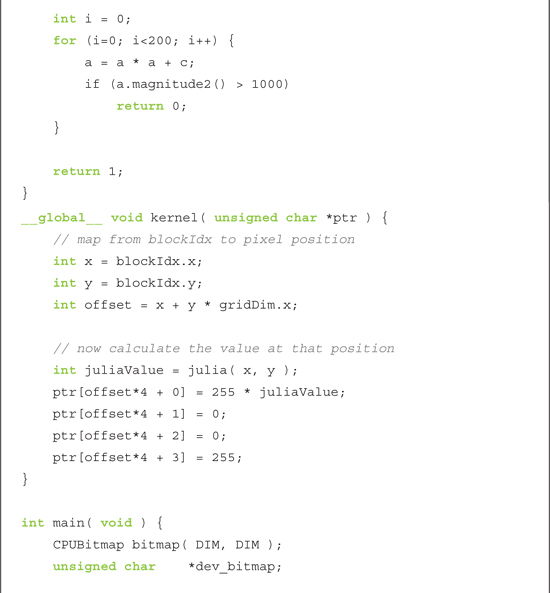
Our main routine is remarkably simple. It creates the appropriate size bitmap image using a utility library provided. Next, it passes a pointer to the bitmap data to the kernel function.
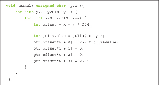
The computation kernel does nothing more than iterate through all points we care to render, calling julia() on each to determine membership in the Julia Set. The function julia() will return 1 if the point is in the set and 0 if it is not in the set. We set the point’s color to be red if julia() returns 1 and black if it returns 0. These colors are arbitrary, and you should feel free to choose a color scheme that matches your personal aesthetics.
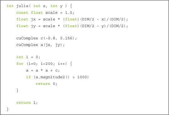
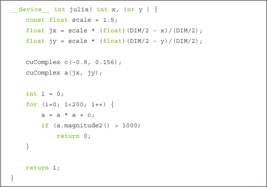
This function is the meat of the example. We begin by translating our pixel coordinate to a coordinate in complex space. To center the complex plane at the image center, we shift by DIM/2. Then, to ensure that the image spans the range of -1.0 to 1.0, we scale the image coordinate by DIM/2. Thus, given an image point at (x,y), we get a point in complex space at ( (DIM/2 – x)/(DIM/2), ((DIM/2 – y)/(DIM/2) ).
Then, to potentially zoom in or out, we introduce a scale factor. Currently, the scale is hard-coded to be 1.5, but you should tweak this parameter to zoom in or out. If you are feeling really ambitious, you could make this a command-line parameter.
After obtaining the point in complex space, we then need to determine whether the point is in or out of the Julia Set. If you recall the previous section, we do this by computing the values of the iterative equation Zn+1 = zn2 + C. Since C is some arbitrary complex-valued constant, we have chosen -0.8 + 0.156i because it happens to yield an interesting picture. You should play with this constant if you want to see other versions of the Julia Set.
In the example, we compute 200 iterations of this function. After each iteration, we check whether the magnitude of the result exceeds some threshold (1,000 for our purposes). If so, the equation is diverging, and we can return 0 to indicate that the point is not in the set. On the other hand, if we finish all 200 iterations and the magnitude is still bounded under 1,000, we assume that the point is in the set, and we return 1 to the caller, kernel().
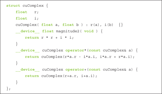
Since all the computations are being performed on complex numbers, we define a generic structure to store complex numbers.
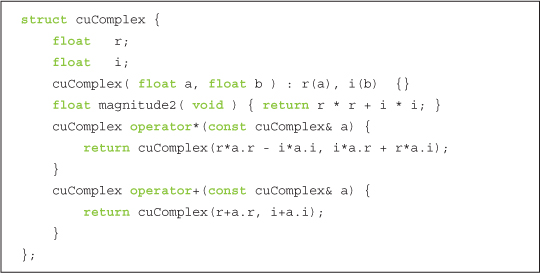
The structure represents complex numbers with two data elements: a single-precision real component r and a single-precision imaginary component i. The structure defines addition and multiplication operators that combine complex numbers as expected. (If you are completely unfamiliar with complex numbers, you can get a quick primer online.) Finally, we define a method that returns the magnitude of the complex number.
GPU Julia Set
The device implementation is remarkably similar to the CPU version, continuing a trend you may have noticed.
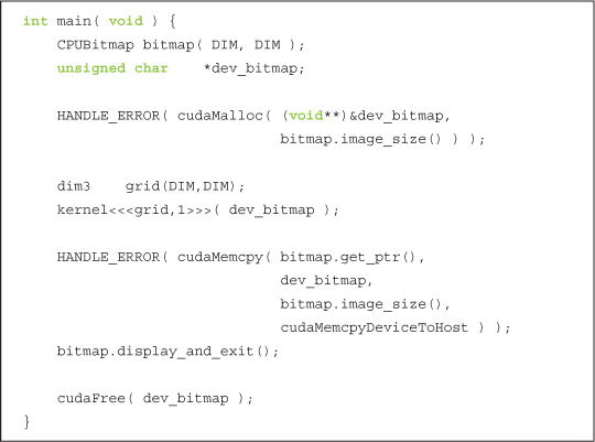
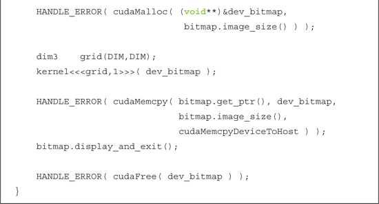
This version of main() looks much more complicated than the CPU version, but the flow is actually identical. Like with the CPU version, we create a DIM x DIM bitmap image using our utility library. But because we will be doing computation on a GPU, we also declare a pointer called dev_bitmap to hold a copy of the data on the device. And to hold data, we need to allocate memory using cudaMalloc().
We then run our kernel() function exactly like in the CPU version, although now it is a __global__ function, meaning it will run on the GPU. As with the CPU example, we pass kernel() the pointer we allocated in the previous line to store the results. The only difference is that the memory resides on the GPU now, not on the host system.
The most significant difference is that we specify how many parallel blocks on which to execute the function kernel(). Because each point can be computed independently of every other point, we simply specify one copy of the function for each point we want to compute. We mentioned that for some problem domains, it helps to use two-dimensional indexing. Unsurprisingly, computing function values over a two-dimensional domain such as the complex plane is one of these problems. So, we specify a two-dimensional grid of blocks in this line:
dim3 grid(DIM,DIM);
The type dim3 is not a standard C type, lest you feared you had forgotten some key pieces of information. Rather, the CUDA runtime header files define some convenience types to encapsulate multidimensional tuples. The type dim3 represents a three-dimensional tuple that will be used to specify the size of our launch. But why do we use a three-dimensional value when we oh-so-clearly stated that our launch is a two-dimensional grid?
Frankly, we do this because a three-dimensional, dim3 value is what the CUDA runtime expects. Although a three-dimensional launch grid is not currently supported, the CUDA runtime still expects a dim3 variable where the last component equals 1. When we initialize it with only two values, as we do in the statement dim3 grid(DIM,DIM), the CUDA runtime automatically fills the third dimension with the value 1, so everything here will work as expected. Although it’s possible that NVIDIA will support a three-dimensional grid in the future, for now we’ll just play nicely with the kernel launch API because when coders and APIs fight, the API always wins.
We then pass our dim3 variable grid to the CUDA runtime in this line:
kernel<<<grid,1>>>( dev _ bitmap );
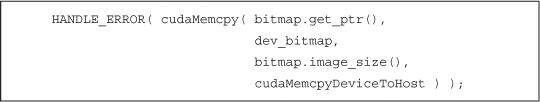
Finally, a consequence of the results residing on the device is that after executing kernel(), we have to copy the results back to the host. As we learned in previous chapters, we accomplish this with a call to cudaMemcpy(), specifying the direction cudaMemcpyDeviceToHost as the last argument.
One of the last wrinkles in the difference of implementation comes in the implementation of kernel().
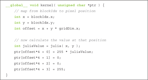
First, we need kernel() to be declared as a __global__ function so it runs on the device but can be called from the host. Unlike the CPU version, we no longer need nested for() loops to generate the pixel indices that get passed to julia(). As with the vector addition example, the CUDA runtime generates these indices for us in the variable blockIdx. This works because we declared our grid of blocks to have the same dimensions as our image, so we get one block for each pair of integers (x,y) between (0,0) and (DIM-1, DIM-1).
Next, the only additional information we need is a linear offset into our output buffer, ptr. This gets computed using another built-in variable, gridDim. This variable is a constant across all blocks and simply holds the dimensions of the grid that was launched. In this example, it will always be the value (DIM, DIM). So, multiplying the row index by the grid width and adding the column index will give us a unique index into ptr that ranges from 0 to (DIM*DIM-1).
![]()
Finally, we examine the actual code that determines whether a point is in or out of the Julia Set. This code should look identical to the CPU version, continuing a trend we have seen in many examples now.
Again, we define a cuComplex structure that defines a method for storing a complex number with single-precision floating-point components. The structure also defines addition and multiplication operators as well as a function to return the magnitude of the complex value.
Notice that we use the same language constructs in CUDA C that we use in our CPU version. The one difference is the qualifier __device__, which indicates that this code will run on a GPU and not on the host. Recall that because these functions are declared as __device__ functions, they will be callable only from other __device__ functions or from __global__ functions.
Since we’ve interrupted the code with commentary so frequently, here is the entire source listing from start to finish:

When you run the application, you should see a visualization of the Julia Set. To convince you that it has earned the title “A Fun Example,” Figure 4.2 shows a screenshot taken from this application.
Figure 4.2 A screenshot from the GPU Julia Set application

4.3 Chapter Review
Congratulations, you can now write, compile, and run massively parallel code on a graphics processor! You should go brag to your friends. And if they are still under the misconception that GPU computing is exotic and difficult to master, they will be most impressed. The ease with which you accomplished it will be our secret. If they’re people you trust with your secrets, suggest that they buy the book, too.
We have so far looked at how to instruct the CUDA runtime to execute multiple copies of our program in parallel on what we called blocks. We called the collection of blocks we launch on the GPU a grid. As the name might imply, a grid can be either a one- or two-dimensional collection of blocks. Each copy of the kernel can determine which block it is executing with the built-in variable blockIdx. Likewise, it can determine the size of the grid by using the built-in variable gridDim. Both of these built-in variables proved useful within our kernel to calculate the data index for which each block is responsible.