
Chapter 7 Texture Memory
When we looked at constant memory, we saw how exploiting special memory spaces under the right circumstances can dramatically accelerate applications. We also learned how to measure these performance gains in order to make informed decisions about performance choices. In this chapter, we will learn about how to allocate and use texture memory. Like constant memory, texture memory is another variety of read-only memory that can improve performance and reduce memory traffic when reads have certain access patterns. Although texture memory was originally designed for traditional graphics applications, it can also be used quite effectively in some GPU computing applications.
7.1 Chapter Objectives
Through the course of this chapter, you will accomplish the following:
• You will learn about the performance characteristics of texture memory.
• You will learn how to use one-dimensional texture memory with CUDA C.
• You will learn how to use two-dimensional texture memory with CUDA C.
7.2 Texture Memory Overview
If you read the introduction to this chapter, the secret is already out: There is yet another type of read-only memory that is available for use in your programs written in CUDA C. Readers familiar with the workings of graphics hardware will not be surprised, but the GPU’s sophisticated texture memory may also be used for general-purpose computing. Although NVIDIA designed the texture units for the classical OpenGL and DirectX rendering pipelines, texture memory has some properties that make it extremely useful for computing.
Like constant memory, texture memory is cached on chip, so in some situations it will provide higher effective bandwidth by reducing memory requests to off-chip DRAM. Specifically, texture caches are designed for graphics applications where memory access patterns exhibit a great deal of spatial locality. In a computing application, this roughly implies that a thread is likely to read from an address “near” the address that nearby threads read, as shown in Figure 7.1.
Figure 7.1 A mapping of threads into a two-dimensional region of memory
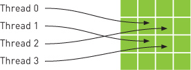
Arithmetically, the four addresses shown are not consecutive, so they would not be cached together in a typical CPU caching scheme. But since GPU texture caches are designed to accelerate access patterns such as this one, you will see an increase in performance in this case when using texture memory instead of global memory. In fact, this sort of access pattern is not incredibly uncommon in general-purpose computing, as we shall see.
7.3 Simulating Heat Transfer
Physical simulations can be among the most computationally challenging problems to solve. Fundamentally, there is often a trade-off between accuracy and computational complexity. As a result, computer simulations have become more and more important in recent years, thanks in large part to the increased accuracy possible as a consequence of the parallel computing revolution. Since many physical simulations can be parallelized quite easily, we will look at a very simple simulation model in this example.
7.3.1 Simple Heating Model
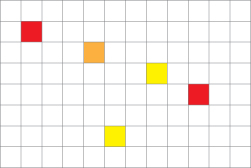
To demonstrate a situation where you can effectively employ texture memory, we will construct a simple two-dimensional heat transfer simulation. We start by assuming that we have some rectangular room that we divide into a grid. Inside the grid, we will randomly scatter a handful of “heaters” with various fixed temperatures. Figure 7.2 shows an example of what this room might look like.
Figure 7.2 A room with “heaters” of various temperature
Given a rectangular grid and configuration of heaters, we are looking to simulate what happens to the temperature in every grid cell as time progresses. For simplicity, cells with heaters in them always remain at a constant temperature. At every step in time, we will assume that heat “flows” between a cell and its neighbors. If a cell’s neighbor is warmer than it is, the warmer neighbor will tend to warm it up. Conversely, if a cell has a neighbor cooler than it is, it will cool off. Qualitatively, Figure 7.3 represents this flow of heat.
Figure 7.3 Heat dissipating from warm cells into cold cells

In our heat transfer model, we will compute the new temperature in a grid cell as a sum of the differences between its temperature and the temperatures of its neighbors, or, essentially, an update equation as shown in Equation 7.1.
![]()
In the equation for updating a cell’s temperature, the constant k simply represents the rate at which heat flows through the simulation. A large value of k will drive the system to a constant temperature quickly, while a small value will allow the solution to retain large temperature gradients longer. Since we consider only four neighbors (top, bottom, left, right) and k and TOLD remain constant in the equation, this update becomes like the one shown in Equation 7.2.
![]()
Like with the ray tracing example in the previous chapter, this model is not intended to be close to what might be used in industry (in fact, it is not really even an approximation of something physically accurate). We have simplified this model immensely in order to draw attention to the techniques at hand. With this in mind, let’s take a look at how the update given by Equation 7.2 can be computed on the GPU.
7.3.2 Computing Temperature Updates
We will cover the specifics of each step in a moment, but at a high level, our update process proceeds as follows:
1. Given some grid of input temperatures, copy the temperature of cells with heaters to this grid. This will overwrite any previously computed temperatures in these cells, thereby enforcing our restriction that “heating cells” remain at a constant temperature. This copy gets performed in copy_const_kernel().
2. Given the input temperature grid, compute the output temperatures based on the update in Equation 7.2. This update gets performed in blend_kernel().
3. Swap the input and output buffers in preparation of the next time step. The output temperature grid computed in step 2 will become the input temperature grid that we start with in step 1 when simulating the next time step.
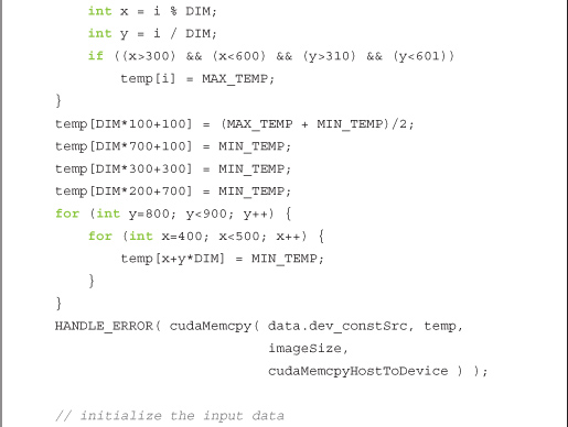
Before beginning the simulation, we assume we have generated a grid of constants. Most of the entries in this grid are zero, but some entries contain nonzero temperatures that represent heaters at fixed temperatures. This buffer of constants will not change over the course of the simulation and gets read at each time step.
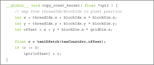
Because of the way we are modeling our heat transfer, we start with the output grid from the previous time step. Then, according to step 1, we copy the temperatures of the cells with heaters into this output grid, overwriting any previously computed temperatures. We do this because we have assumed that the temperature of these heater cells remains constant. We perform this copy of the constant grid onto the input grid with the following kernel:
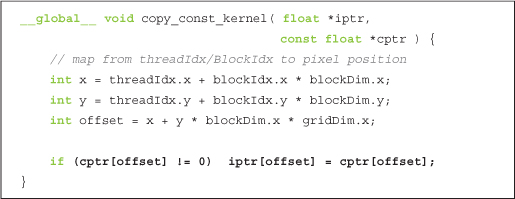
The first three lines should look familiar. The first two lines convert a thread’s threadIdx and blockIdx into an x- and a y-coordinate. The third line computes a linear offset into our constant and input buffers. The highlighted line performs the copy of the heater temperature in cptr[] to the input grid in iptr[]. Notice that the copy is performed only if the cell in the constant grid is nonzero. We do this to preserve any values that were computed in the previous time step within cells that do not contain heaters. Cells with heaters will have nonzero entries in cptr[] and will therefore have their temperatures preserved from step to step thanks to this copy kernel.
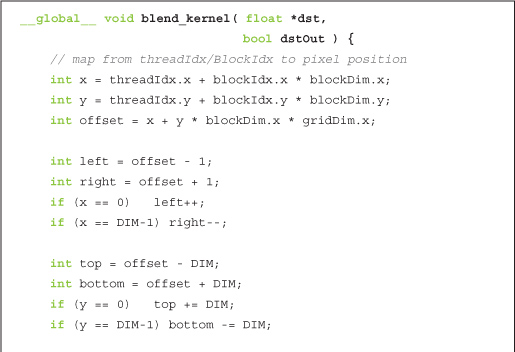
Step 2 of the algorithm is the most computationally involved. To perform the updates, we can have each thread take responsibility for a single cell in our simulation. Each thread will read its cell’s temperature and the temperatures of its neighboring cells, perform the previous update computation, and then update its temperature with the new value. Much of this kernel resembles techniques you’ve used before.
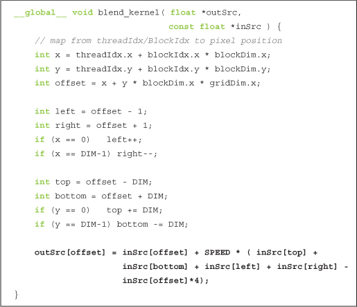
Notice that we start exactly as we did for the examples that produced images as their output. However, instead of computing the color of a pixel, the threads are computing temperatures of simulation grid cells. Nevertheless, they start by converting their threadIdx and blockIdx into an x, y, and offset. You might be able to recite these lines in your sleep by now (although for your sake, we hope you aren’t actually reciting them in your sleep).
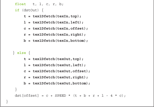
Next, we determine the offsets of our left, right, top, and bottom neighbors so that we can read the temperatures of those cells. We will need those values to compute the updated temperature in the current cell. The only complication here is that we need to adjust indices on the border so that cells around the edges do not wrap around. Finally, in the highlighted line, we perform the update from Equation 7.2, adding the old temperature and the scaled differences of that temperature and the cell’s neighbors’ temperatures.
7.3.3 Animating the Simulation
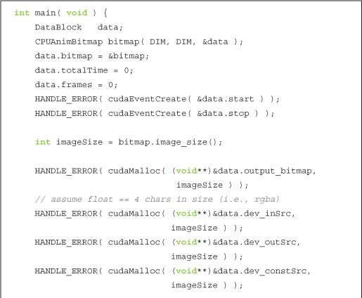
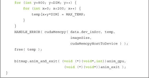
The remainder of the code primarily sets up the grid and then displays an animated output of the heat map. We will walk through that code now:
We have equipped the code with event-based timing as we did in the previous chapter’s ray tracing example. The timing code serves the same purpose as it did previously. Since we will endeavor to accelerate the initial implementation, we have put in place a mechanism by which we can measure performance and convince ourselves that we have succeeded.
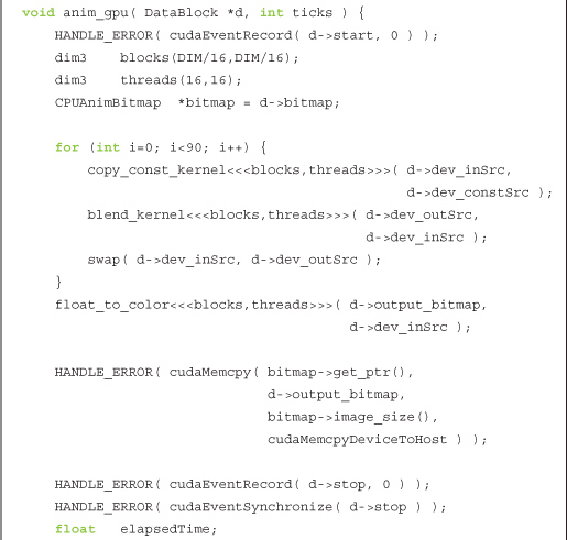
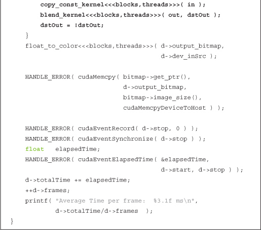
The function anim_gpu() gets called by the animation framework on every frame. The arguments to this function are a pointer to a DataBlock and the number of ticks of the animation that have elapsed. As with the animation examples, we use blocks of 256 threads that we organize into a two-dimensional grid of 16 x 16. Each iteration of the for() loop in anim_gpu() computes a single time step of the simulation as described by the three-step algorithm at the beginning of Section 7.3.2: Computing Temperature Updates. Since the DataBlock contains the constant buffer of heaters as well as the output of the last time step, it encapsulates the entire state of the animation, and consequently, anim_gpu() does not actually need to use the value of ticks anywhere.
You will notice that we have chosen to do 90 time steps per frame. This number is not magical but was determined somewhat experimentally as a reasonable trade-off between having to download a bitmap image for every time step and computing too many time steps per frame, resulting in a jerky animation. If you were more concerned with getting the output of each simulation step than you were with animating the results in real time, you could change this such that you computed only a single step on each frame.
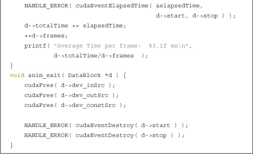
After computing the 90 time steps since the previous frame, anim_gpu() is ready to copy a bitmap frame of the current animation back to the CPU. Since the for() loop leaves the input and output swapped, we pass the input buffer to the next kernel,, which actually contains the output of the 90th time step. We convert the temperatures to colors using the kernel float_to_color() and then copy the resultant image back to the CPU with a cudaMemcpy() that specifies the direction of copy as cudaMemcpyDeviceToHost. Finally, to prepare for the next sequence of time steps, we swap the output buffer back to the input buffer since it will serve as input to the next time steps.
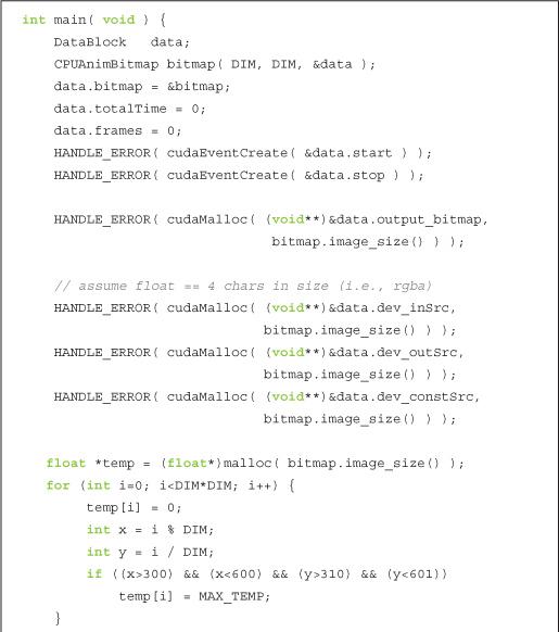
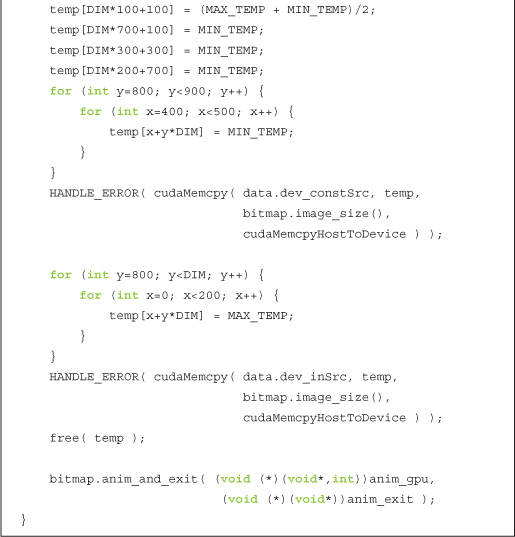
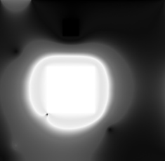
Figure 7.4 shows an example of what the output might look like. You will notice in the image some of the “heaters” that appear to be pixel-sized islands that disrupt the continuity of the temperature distribution.
Figure 7.4 A screenshot from the animated heat transfer simulation
7.3.4 Using Texture Memory
There is a considerable amount of spatial locality in the memory access pattern required to perform the temperature update in each step. As we explained previously, this is exactly the type of access pattern that GPU texture memory is designed to accelerate. Given that we want to use texture memory, we need to learn the mechanics of doing so.
First, we will need to declare our inputs as texture references. We will use references to floating-point textures, since our temperature data is floating-point.
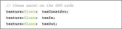
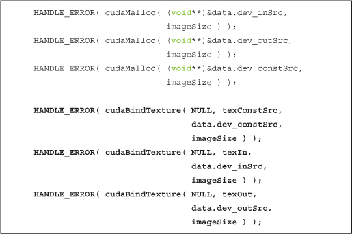
The next major difference is that after allocating GPU memory for these three buffers, we need to bind the references to the memory buffer using cudaBindTexture(). This basically tells the CUDA runtime two things:
• We intend to use the specified buffer as a texture.
• We intend to use the specified texture reference as the texture’s “name.”
After the three allocations in our heat transfer simulation, we bind the three allocations to the texture references declared earlier (texConstSrc, texIn, and texOut).
At this point, our textures are completely set up, and we’re ready to launch our kernel. However, when we’re reading from textures in the kernel, we need to use special functions to instruct the GPU to route our requests through the texture unit and not through standard global memory. As a result, we can no longer simply use square brackets to read from buffers; we need to modify blend_kernel() to use tex1Dfetch() when reading from memory.
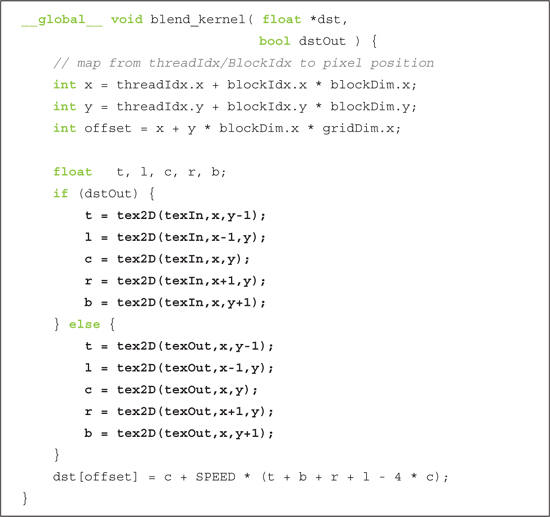
Additionally, there is another difference between using global and texture memory that requires us to make another change. Although it looks like a function, tex1Dfetch() is a compiler intrinsic. And since texture references must be declared globally at file scope, we can no longer pass the input and output buffers as parameters to blend_kernel() because the compiler needs to know at compile time which textures tex1Dfetch() should be sampling. Rather than passing pointers to input and output buffers as we previously did, we will pass to blend_kernel() a boolean flag dstOut that indicates which buffer to use as input and which to use as output. The changes to blend_kernel() are highlighted here:
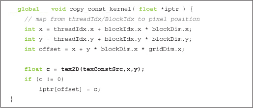
Since the copy_const_kernel() kernel reads from our buffer that holds the heater positions and temperatures, we will need to make a similar modification there in order to read through texture memory instead of global memory:
Since the signature of blend_kernel() changed to accept a flag that switches the buffers between input and output, we need a corresponding change to the anim_gpu() routine. Rather than swapping buffers, we set dstOut = !dstOut to toggle the flag after each series of calls:

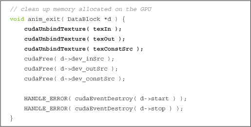
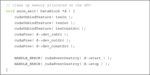
The final change to our heat transfer routine involves cleaning up at the end of the application’s run. Rather than just freeing the global buffers, we also need to unbind textures:
7.3.5 Using Two-Dimensional Texture Memory
Toward the beginning of this book, we mentioned how some problems have two-dimensional domains, and therefore it can be convenient to use two-dimensional blocks and grids at times. The same is true for texture memory. There are many cases when having a two-dimensional memory region can be useful, a claim that should come as no surprise to anyone familiar with multidimensional arrays in standard C. Let’s look at how we can modify our heat transfer application to use two-dimensional textures.
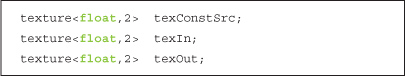
First, our texture reference declarations change. If unspecified, texture references are one-dimensional by default, so we add a dimensionality argument of 2 in order to declare two-dimensional textures.
The simplification promised by converting to two-dimensional textures comes in the blend_kernel() method. Although we need to change our tex1Dfetch() calls to tex2D() calls, we no longer need to use the linearized offset variable to compute the set of offsets top, left, right, and bottom. When we switch to a two-dimensional texture, we can use x and y directly to address the texture.
Furthermore, we no longer have to worry about bounds overflow when we switch to using tex2D(). If one of x or y is less than zero, tex2D() will return the value at zero. Likewise, if one of these values is greater than the width, tex2D() will return the value at width 1. Note that in our application, this behavior is ideal, but it’s possible that other applications would desire other behavior.
As a result of these simplifications, our kernel cleans up nicely.
Since all of our previous calls to tex1Dfetch() need to be changed to tex2D() calls, we make the corresponding change in copy_const_kernel(). Similarly to the kernel blend_kernel(), we no longer need to use offset to address the texture; we simply use x and y to address the constant source:
The final change to the one-dimensional texture version of our heat transfer simulation is along the same lines as our previous changes. Specifically, in main(), we need to change our texture binding calls to instruct the runtime that the buffer we plan to use will be treated as a two-dimensional texture, not a one-dimensional one:
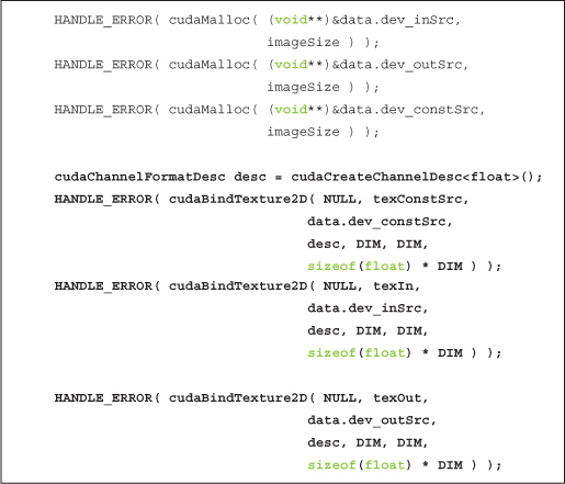
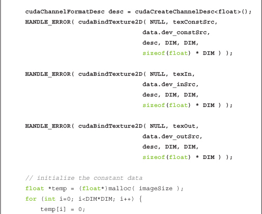
As with the nontexture and one-dimensional texture versions, we begin by allocating storage for our input arrays. We deviate from the one-dimensional example because the CUDA runtime requires that we provide a cudaChannelFormatDesc when we bind two-dimensional textures. The previous listing includes a declaration of a channel format descriptor. In our case, we can accept the default parameters and simply need to specify that we require a floating-point descriptor. We then bind the three input buffers as two-dimensional textures using cudaBindTexture2D(), the dimensions of the texture (DIM x DIM), and the channel format descriptor (desc). The rest of main() remains the same.
Although we needed different functions to instruct the runtime to bind one-dimensional or two-dimensional textures, we use the same routine to unbind the texture, cudaUnbindTexture(). Because of this, our cleanup routine can remain unchanged.
The version of our heat transfer simulation that uses two-dimensional textures has essentially identical performance characteristics as the version that uses one-dimensional textures. So from a performance standpoint, the decision between one- and two-dimensional textures is likely to be inconsequential. For our particular application, the code is a little simpler when using two-dimensional textures because we happen to be simulating a two-dimensional domain. But in general, since this is not always the case, we suggest you make the decision between one- and two-dimensional textures on a case-by-case basis.
7.4 Chapter Review
As we saw in the previous chapter with constant memory, some of the benefit of texture memory comes as the result of on-chip caching. This is especially noticeable in applications such as our heat transfer simulation: applications that have some spatial coherence to their data access patterns. We saw how either one- or two-dimensional textures can be used, both having similar performance characteristics. As with a block or grid shape, the choice of one- or two-dimensional texture is largely one of convenience. Since the code became somewhat cleaner when we switched to two-dimensional textures and the borders are handled automatically, we would probably advocate the use of a 2D texture in our heat transfer application. But as you saw, it will work fine either way.
Texture memory can provide additional speedups if we utilize some of the conversions that texture samplers can perform automatically, such as unpacking packed data into separate variables or converting 8- and 16-bit integers to normalized floating-point numbers. We didn’t explore either of these capabilities in the heat transfer application, but they might be useful to you!