
Continuity
In This Chapter
![]()
- What it means to be continuous
- Classifying discontinuity
- When discontinuity is removable
- The Intermediate Value Theorem
Now that you understand and can evaluate limits, it’s time to move forward with that knowledge. Flip through any calculus textbook and read some of the most important calculus theorems, and you’ll find that nearly every one contains a significant condition: continuity. In fact, almost none of our most important calculus conclusions (including the Fundamental Theorem of Calculus, which sounds pretty darn important) work if the functions in question are not continuous.
Testing for continuity on a function is very similar to testing for the existence of limits on a function. Just as three stipulations must be met in order for a limit to exist at a given point (left- and right-hand limits existing and being equal), three different stipulations must be met in order for a function to be continuous at a point. Just as there are three major cases in which limits do not exist, there are three major causes that force a function to be discontinuous.
Calculus is handy like that—if you look hard enough, you can usually see how one topic flows into the next. Without limits, there’d be no continuity; without continuity, there’d be no derivatives; without derivatives, no integrals; and without integrals, no sleepless, panicked nights trying to cram for calculus tests.
What Does Continuity Look Like?
First of all, let’s set our language straight. Continuous is an adjective that describes a function meeting very specific standards. Just as Boy Scouts must pass tests to earn merit badges, there are three tests a function must pass at any given point in order to earn the “Continuous” merit badge.
Before we get into the nitty-gritty of the math definition, let’s approach continuity from a visual perspective. It is easiest to determine whether or not a function is continuous by looking at its graph. If the graph has no holes, breaks, or jumps, then we can rest assured that the function is continuous. A continuous function is simply a nice, smooth function that can be drawn completely without lifting your pencil. With this intuitive definition in mind, study Figure 7.1. Can you tell which of the following three functions is continuous?
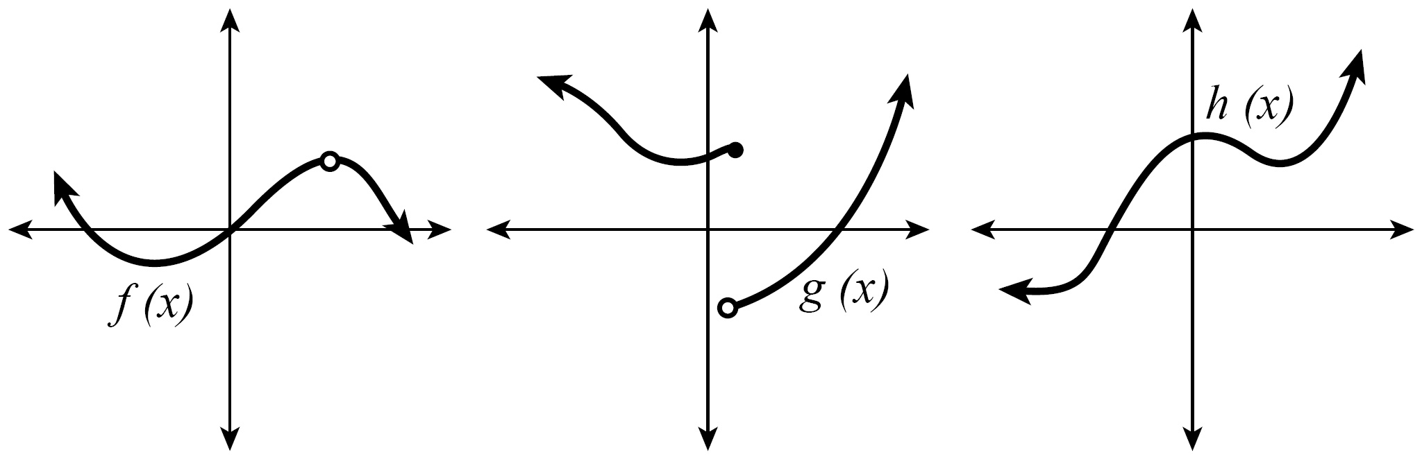
Figure 7.1
One of these things is not like the others; one of these things just doesn’t belong. Which is the continuous function?
Critical Point
A continuous function is like a well-built roller coaster track—no gaps, holes, or breaks means safe riding for its passengers.
Of these functions, only h(x) can be drawn with a single, unbroken pen stroke. The other functions are much more unpredictable: f has an unexpected hole in it, and g suddenly breaks without warning. Only good old h provides a nice smooth ride from start to finish. Function h is like the good, solid, dependable boyfriend or girlfriend you wouldn’t be embarrassed to bring home to Mom and Dad, and the fact that it guarantees no unexpected breakups means peace of mind for your emotional well-being.
The Mathematical Definition of Continuity
The mathematical definition of continuity makes a lot of sense if you keep one thing in mind: whereas limits told us where a function intended to go, continuity guarantees that the function actually made it there. As the saying goes, “The road to hell is paved with good intentions.”
Continuity has the mathematical role of policeman, determining whether or not the function followed through with its intentions (meaning it is continuous) or not (making the function discontinuous).
Many functions are guaranteed to be continuous at each point in their domain, including polynomial, radical, exponential, logarithmic, rational, and trigonometric functions. Most of the discontinuous functions you’ll encounter will be due to undefined spots in rational functions and jumps due to piecewise-defined functions. We’ll discuss more about specific causes of discontinuity in the next section.
Critical Point
A function is continuous at a point if the limit and function value there are equal. In other words, the limit exists if the intended height matches the actual function height.
With that in mind, here is the official definition of continuity:
A function f(x) is continuous at a point x = c if the following three conditions are met:
 exists
- f(c) is defined
In other words, the limit exists at x = c (which means the function has an intended height); the function exists at x = c (which means that there is no hole there); and the limit is equal to the function value (i.e., the function’s value matches its intended value). (By the way, if a function is continuous, you can evaluate any limit on that function using the substitution method, since the function’s value at any point will be equal to the limit there.)
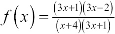
Example 1: Explain why the function f(x), defined here, is continuous at x = –3.
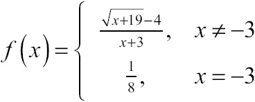
Solution: To test for continuity, you must find the limit and the function value at x = –3 (and make sure they are equal). Now, that’s one ugly function. How can you determine its intended height (limit) at x = –3? Clearly, the top rule in this piecewise-defined function governs the function’s value for every single x except for x = –3. When you are finding a limit, you want to see what height is intended as you approach x = –3, not the value actually reached at x = –3, so you’ll find the limit of the larger, ugly, top rule for f. Use the conjugate method:
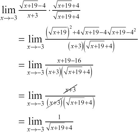
Whew! Now that (x + 3) no longer appears in the denominator, you can apply the substitution method:
The limit clearly exists when x = –3, and it is equal to ![]() . The first condition of continuity is satisfied. Now, on to the second. According to the function’s definition, you know that
. The first condition of continuity is satisfied. Now, on to the second. According to the function’s definition, you know that ![]() , so the function does exist there. Therefore, you can conclude that the function is continuous at x = –3, because the limit is equal to the function value there.
, so the function does exist there. Therefore, you can conclude that the function is continuous at x = –3, because the limit is equal to the function value there.
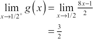
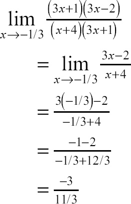
Example 2: Determine whether the function g(x), defined here, is continuous at ![]() :
:
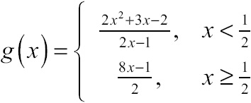
Solution: If g(x) is continuous at ![]() , three things have to be true: (1)
, three things have to be true: (1) ![]() must exist, (2)
must exist, (2) ![]() must exist, and (3) those values must be equal. The easiest of the three conditions to test is the second one. Calculate
must exist, and (3) those values must be equal. The easiest of the three conditions to test is the second one. Calculate ![]() :
:
So far so good; ![]() exists, but now there’s no avoiding the much more difficult task of determining whether the limit exists there. Notice that the way g(x) is defined changes at
exists, but now there’s no avoiding the much more difficult task of determining whether the limit exists there. Notice that the way g(x) is defined changes at ![]() , which means g(x) may intend to reach two different heights on the graph as you approach from the left and the right. Good news! You have already calculated the right-hand limit using the substitution method:
, which means g(x) may intend to reach two different heights on the graph as you approach from the left and the right. Good news! You have already calculated the right-hand limit using the substitution method:
Evaluating the left-hand limit is a little trickier. You need to employ the factoring method:
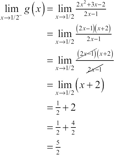
Red alert! The left- and right-hand limits are not equal as x approaches ![]() , because
, because ![]() . If the left- and right-hand limits aren’t equal, then the general limit doesn’t exist at
. If the left- and right-hand limits aren’t equal, then the general limit doesn’t exist at ![]() . That means the first condition of continuity has not been met.
. That means the first condition of continuity has not been met.
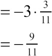
Your goal was to determine whether or not g(x) is continuous when ![]() , and the answer is no. Take a look at the graph of g(x) to visually verify that the function does not intend to reach the same location as you approach
, and the answer is no. Take a look at the graph of g(x) to visually verify that the function does not intend to reach the same location as you approach ![]() from the left and the right.
from the left and the right.
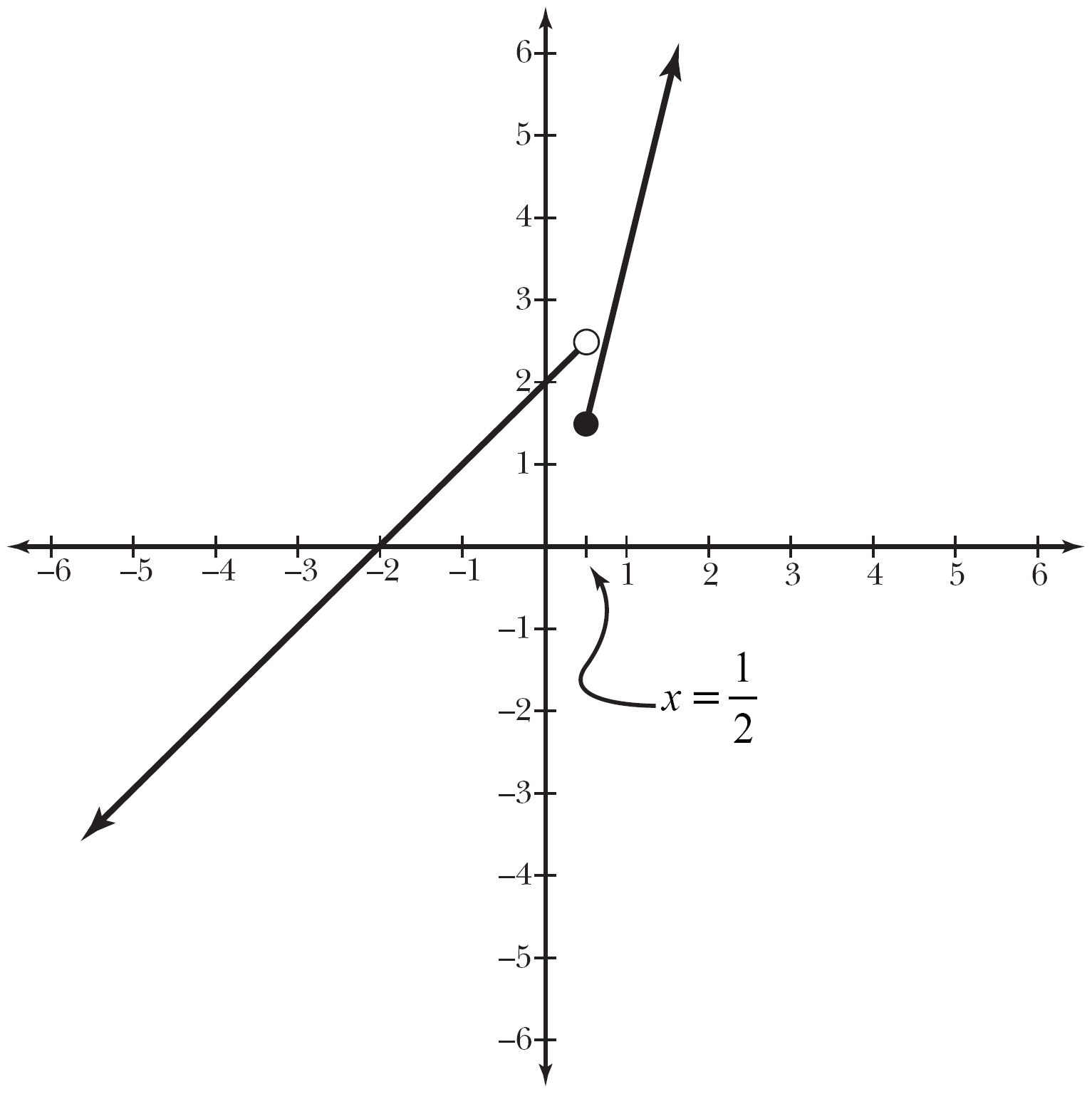
Figure 7.2
Function g(x) is not continuous at ![]() . The graph also helps you decide which expression to use as you approach from the left and the right: the graph of
. The graph also helps you decide which expression to use as you approach from the left and the right: the graph of ![]() is left of
is left of ![]() and the graph of
and the graph of ![]() is right of
is right of ![]() .
.
A function cannot be continuous at an x-value where a limit does not exist; g(x) is discontinuous at ![]() due to a jump discontinuity. Are you asking yourself, “What’s a jump discontinuity?” If so, I’m glad you asked. If not, play along and pretend you did. Either way, I’ll meet you in the next section to explain what I mean.
due to a jump discontinuity. Are you asking yourself, “What’s a jump discontinuity?” If so, I’m glad you asked. If not, play along and pretend you did. Either way, I’ll meet you in the next section to explain what I mean.
You’ve got problems
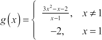
Problem 1: Determine whether or not the function g(x), defined here, is continuous at x = 1.
Not much happens in the life of a graph—it lives in a happy little domain, playing matchmaker to pairs of coordinates. However, there are three things that can happen over the span of a function which change it fundamentally, making it discontinuous. Memorizing the three major causes of discontinuity is not so important; instead, recognize exactly what causes the function to fall short of continuity’s requirements.
Jump Discontinuity
A jump discontinuity is typically caused by a piecewise-defined function whose pieces don’t meet neatly, leaving gaping tears in the graph large enough for an elephant, or other tusked mammal, to walk through. Consider the function:
This graph is made up of two linear pieces, and the rule governing the function changes when x = 0. Look at the graph of f(x) in Figure 7.3.
Definition
A jump discontinuity occurs when no general limit exists at the given x value (because the right- and left-hand limits exist but are not equal). A function is everywhere continuous if it is continuous for each x in its domain.
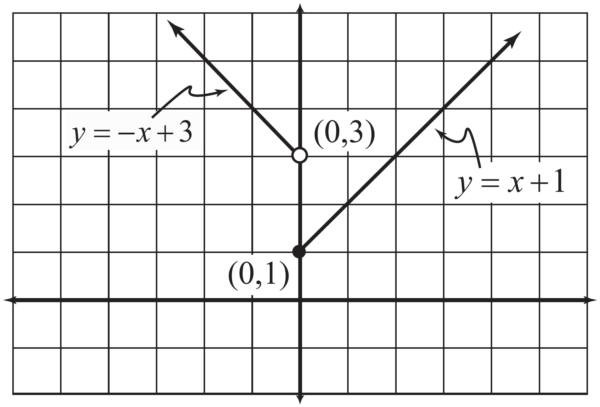
Figure 7.3
The graph of f(x) exhibits an unhealthy dual personality since it is defined by a piecewise-defined function.
When x = 0, the graph has a tragic and unsightly break. Whereas the left-hand piece is heading toward a height of y = 3 as you approach x = 0, the right-hand piece has a height of y = 1 when x = 0. Does this sound familiar? It should: the left- and right-hand limits are unequal at x = 0, so ![]() does not exist. This breaks the first rule requirement of continuity, rendering f(x) discontinuous.
does not exist. This breaks the first rule requirement of continuity, rendering f(x) discontinuous.
In the next example, you are given a piecewise-defined function. Your goal is to shield it from the same fate as the pitiful function f(x) by choosing a value for the constant c that ensures that the pieces of the graph will meet when the defining function rule changes. Godspeed!
Example 3: Given h(x) as defined here, calculate the real number c that makes h(x) everywhere continuous:
Solution: The top rule in h(x) will define the function for all numbers less than or equal to 3, and its reign ends once x reaches that boundary. At that point, h(x) will have reached a height of h(3) = 3 – 2 = 1. Therefore, the next rule (x2 + c) must start at exactly that height when x = 3, even though it is technically defined only when x > 3. That’s the key: both pieces must reach the exact same intended height when the graph of a piecewise-defined function changes rules. Thus, when x = 3:
x2 + c = 1
Plug in that x value and solve for c:
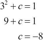
Thus, the second piece of g(x) must be x2 – 8 in order for h(x) to be continuous. You can verify the solution with the graph of h(x) (as shown in Figure 7.4)—no jump discontinuity anywhere to be found.
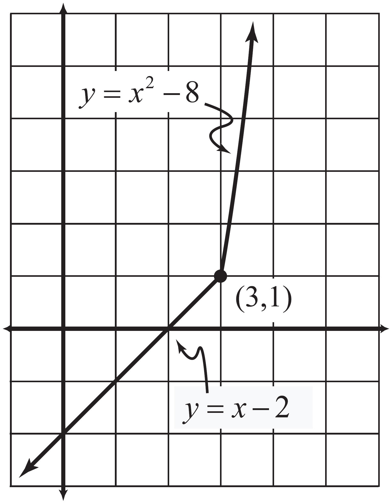
Figure 7.4
The graph of h(x) is nice and continuous now—the pieces of the graph join together seamlessly.
Example 4: Given the function q(x) defined here, calculate the values of a and b that ensure q(x) is continuous for all real numbers. Verify your answers with a graph of q(x).
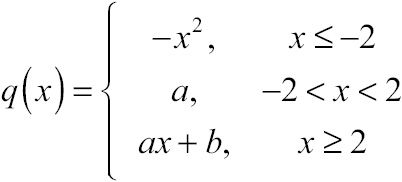
Solution: The individual pieces of function q(x) are each continuous over their domains. The graphs of y = –x2 (a parabola), y = a (a horizontal line at height a), and y = ax + b (a line with slope a and y-intercept b) are unbroken and free of jump discontinuities. Of course, this is a piecewise-defined function, so each of the pieces need to meet when x = –2 and x = 2 if the overall function is going to be continuous. You need to pay special attention to these x-values, where the rules that define the function change.
Let’s start with x = –2. If you substitute that value into –x2, you calculate the left-hand limit of q(x) as x approaches –2.
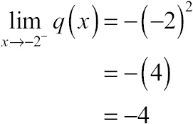
The right-hand limit at x = –2 must be equal to the left-hand limit for the general limit to exist. The right-hand limit is simply the constant a. If the right- and left-hand limits are equal, you can conclude that a also equals –4.
Not only is a = –4 the limit as you approach x = –2 from the right, it is also the limit as you approach x = 2 from the left:
In order for a limit to exist at x = 2, the right-hand limit must also equal –4:
That right-hand limit is equal to the expression ax + b, when x = 2:
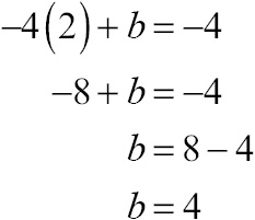
a(2) + b = –4
Recall that a = –4 and solve for b:
Consider the graph of q(x) in Figure 7.5. Notice that there are no jump discontinuities at x = –2 or x = 2.
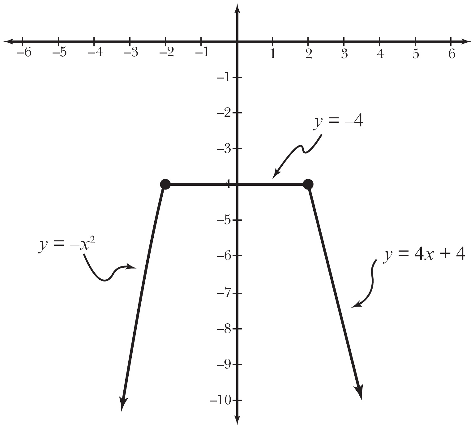
Figure 7.5
The graph of q(x) is continuous for all real numbers, including x = –2 and x = 2.
You’ve got problems
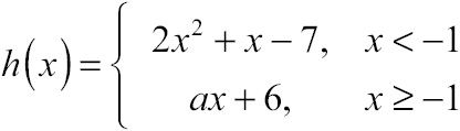
Problem 2: Calculate the value of a that makes the function h(x) everywhere continuous, given:
Point Discontinuity
Point discontinuity occurs when a function contains a hole. Think of it this way: the function is discontinuous only because of that rascally little point, hence the name.
Definition
A point discontinuity occurs when a general limit exists, but the function value is not defined there, breaking the second condition of continuity.
Consider the function ![]() . It is a rational function, so it’s continuous for all points in its domain. Hold on a second, though. The value x = –4 is definitely not in the domain of p(x) (look at the denominator), so p(x) will automatically be discontinuous there. The question is: what sort of discontinuity is present?
. It is a rational function, so it’s continuous for all points in its domain. Hold on a second, though. The value x = –4 is definitely not in the domain of p(x) (look at the denominator), so p(x) will automatically be discontinuous there. The question is: what sort of discontinuity is present?
Classifying the discontinuity in this case is very easy—all you have to do is to test for a limit at that x value. To calculate the limit, use the factoring method:
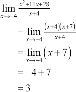
In conclusion, because x = –4 represents a place where p(x) is undefined, and ![]() , you know that there is a hole in the function p(x) at the point (–4,3), a point discontinuity. See the graph of p(x) in Figure 7.6.
, you know that there is a hole in the function p(x) at the point (–4,3), a point discontinuity. See the graph of p(x) in Figure 7.6.
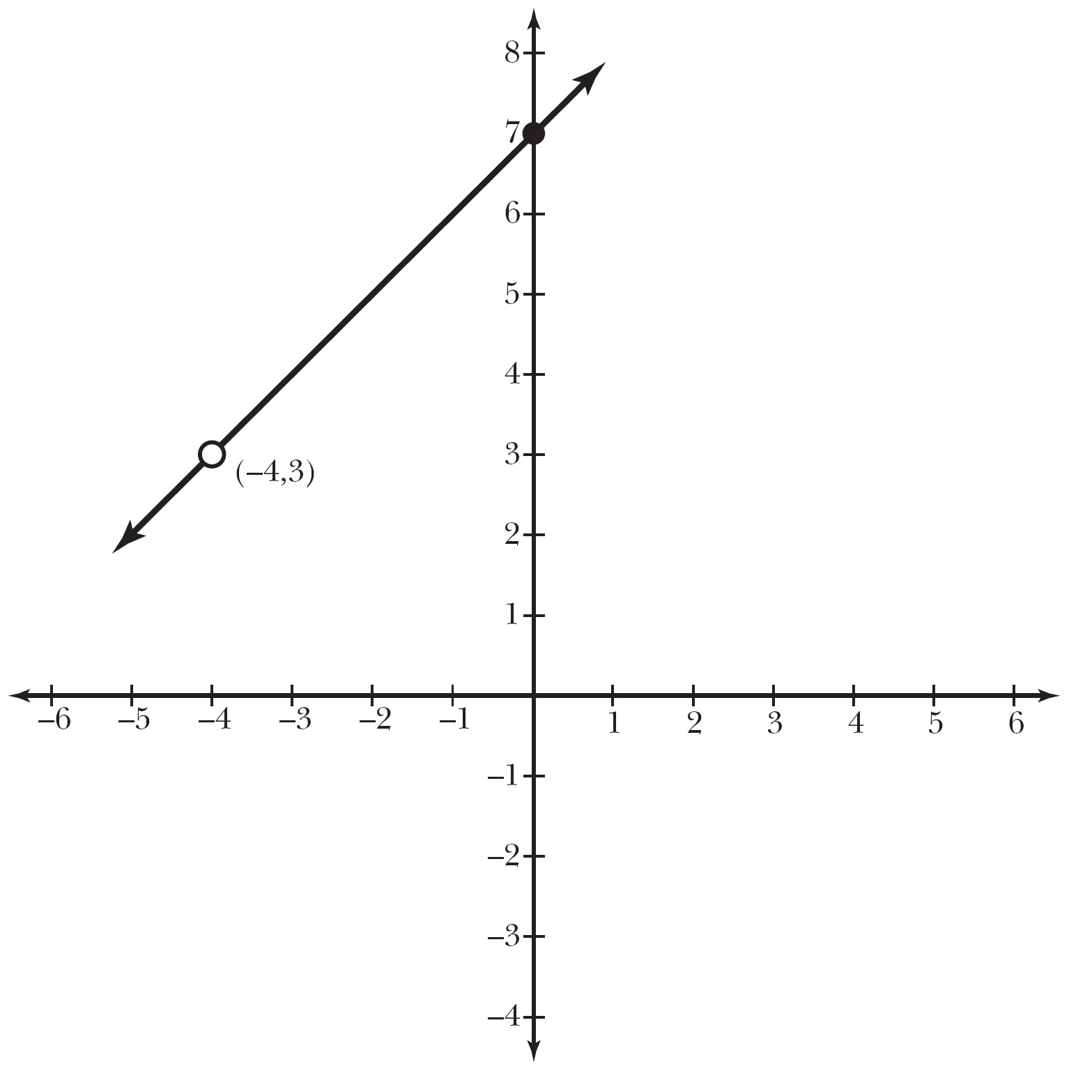
Figure 7.6
The graph of p(x) is also the graph of y = x + 7, except when x = –4, where the function is undefined.
Critical Point
Any x-value for which a function is undefined will automatically be a point of discontinuity for the function. If a limit exists at the point of discontinuity, then it must be a point discontinuity.
Infinite/Essential Discontinuity
An infinite (or essential) discontinuity occurs when a function neither has a limit (because the function increases or decreases without bound) nor is defined at the given x-value. In other words, this type of discontinuity occurs primarily at a vertical asymptote.
Definition
An infinite discontinuity is caused by a vertical asymptote. Since the function increases or decreases without bound, there can be no limit, and since the function never actually touches the asymptote, the function is undefined there. Thus, the presence of a vertical asymptote ruins all the conditions necessary for continuity to occur. Vertical asymptotes are the home wreckers of the continuity world.
It’s easy to determine which x-values cause a vertical asymptote if you remember the shortcut from the last chapter: a function increases or decreases infinitely at a given value of x if substituting that x into the expression results in a constant divided by 0. On the other hand, a result of ![]() usually means that point discontinuity is at work. However, since a result of
usually means that point discontinuity is at work. However, since a result of ![]() doesn’t guarantee you’ve got point discontinuity, you’ll need to double-check to see if the limit exists there. We’ll do this in Example 5, in case you’re confused.
doesn’t guarantee you’ve got point discontinuity, you’ll need to double-check to see if the limit exists there. We’ll do this in Example 5, in case you’re confused.
In summary: if no general limit exists, you have jump discontinuity; if the limit exists but the function doesn’t, you have point discontinuity; if the limit doesn’t exist because it is ∞ or –∞, you have infinite discontinuity.
Now that you’ve got the field guide to discontinuity, let’s look at a typical problem you’ll be given. In it, you’ll be asked either to identify where a function is continuous or, instead, to highlight areas of discontinuity and to classify the type of discontinuity present.
Example 5: Give all x-values for which the function f(x), defined here, is discontinuous, and classify each instance of discontinuity.
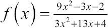
Solution: This is a rational function, so it’s guaranteed to be continuous on its entire domain; the only points you have to inspect are where f(x) is undefined. Because f(x) is rational, it is undefined when its denominator equals 0, and the easiest way to find those locations is by factoring f(x):
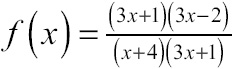
Set the denominator equal to 0 to see that x = –4 and ![]() will be points of discontinuity. Now, we need to explain what kinds of discontinuity they represent. Plug each into f(x). Substituting x = –4 results in
will be points of discontinuity. Now, we need to explain what kinds of discontinuity they represent. Plug each into f(x). Substituting x = –4 results in ![]() , indicating the presence of a vertical asymptote and an infinite discontinuity. However, substituting
, indicating the presence of a vertical asymptote and an infinite discontinuity. However, substituting ![]() into f(x) gives you
into f(x) gives you ![]() , which means there is probably a hole in the function there. That’s not good enough supporting work, however. You need to prove that there’s a hole there in order to conclude that
, which means there is probably a hole in the function there. That’s not good enough supporting work, however. You need to prove that there’s a hole there in order to conclude that ![]() represents a point discontinuity. All the proof you’ll need is to verify the presence of a limit at
represents a point discontinuity. All the proof you’ll need is to verify the presence of a limit at ![]() . To do so, use the factoring method:
. To do so, use the factoring method:
Convert the complex fraction into a regular fraction by multiplying the numerator (–3) by the reciprocal of the denominator ![]() :
:
Because the limit exists, there is a point discontinuity when ![]() . You can verify this with the graph of f(x) in Figure 7.7.
. You can verify this with the graph of f(x) in Figure 7.7.
Figure 7.7
The graph of f(x) has an infinite discontinuity at x = –4 and a point discontinuity at ![]() .
.
You’ve got problems
Problem 3: Give all x-values for which the function here is discontinuous, and classify each instance of discontinuity.
Removable vs. Nonremovable Discontinuity
Occasionally you’ll see a function described as having removable or nonremovable discontinuity. These terms are more specific than simply stating that a function is discontinuous, but less specific than stating that it has point, jump, or infinite discontinuity.
However, because these terms appear often, it’s good to know what they mean. A removable discontinuity is one that could be eliminated by simply redefining a finite number of points. In other words, if you can “fix” the discontinuity by filling in holes, then that discontinuity is removable. Let’s go back to the function we examined in Example 5 for a moment:
Definition
A removable discontinuity occurs at a given x-value if a limit exists there, since you can redefine the function to fill in the holes (and thus remove the discontinuity) if you choose to. Therefore, point and removable discontinuity are essentially synonymous.
This function has a point discontinuity at ![]() , because
, because ![]() . If I redefine f(x) slightly, setting
. If I redefine f(x) slightly, setting ![]() , then the limit equals the function value when
, then the limit equals the function value when ![]() , and f(x) is continuous there. Mathematically, the new function f(x) looks like this:
, and f(x) is continuous there. Mathematically, the new function f(x) looks like this:
You don’t actually have to change the function for it to be removably discontinuous (in fact, if you did change the function, it wouldn’t be discontinuous when ![]() ). However, if it is possible to change a few points in order to fill in the function’s holes, the discontinuities are removable.
). However, if it is possible to change a few points in order to fill in the function’s holes, the discontinuities are removable.
Nonremovable discontinuity occurs when a function has no general limit at the given x-value, as is the case with infinite and jump discontinuities. There is no way to redefine a finite number of points to “repair” this type of discontinuity; the function is fundamentally discontinuous there, and no amount of rehabilitation or mood-altering medication can make this function safe for a cultured society. I gasp at the thought, but not even a charity rock concert can help (sorry, U2). Back to the function f(x) from Example 5 for illustration. Since a vertical asymptote occurs at x = –4 and no general limit exists there, x = –4 represents an instance of nonremovable discontinuity.
Definition
A nonremovable discontinuity occurs at a given x-value if no general limit exists there, making it impossible to remove the discontinuity by redefining a fixed number of points. Jump and infinite discontinuities are both examples of nonremovable discontinuity.
The Intermediate Value Theorem
Break out the party favors—we’ve arrived at our first official calculus theorem.
The Intermediate Value Theorem: If a function f(x) is continuous on the closed interval [a,b], then for every real number d between f(a) and f(b), there exists a real number c between a and b such that f(c) = d.
Now, let me explain what the heck that means using a simple example. Like all red-blooded Americans, I enjoy a little too much holiday dining during the winter months of November and December. If we were to exaggerate my weight gain (a little), it might have the following humorously titled “Kelley’s Date vs. Weight Graph,” which I’ll call w(x) in Figure 7.8.
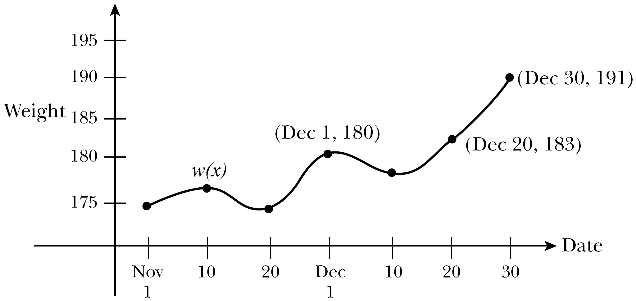
Figure 7.8
Kelley’s Date vs. Weight Graph.
From the graph, we can see that I weighed 180 pounds on December 1 and porked up to 191 by the time December 30 “rolled around,” poor pun definitely intended. Comparing this to the Intermediate Value Theorem, a = Dec 1, b = Dec 30 (weird values, but go with me on this), f(a) = w(Dec 1) = 180, and f(b) = w(Dec 30) = 191. According to the theorem, I can choose any value between 180 and 191 (for example, 183), and I am guaranteed that at some time between December 1 and December 30, I actually weighed that much.
The Intermediate Value Theorem does not claim to tell you where your function reaches that value or how many times it does. The theorem simply claims (in a calm, soothing voice) that every height a function reaches on a specific x-interval boundary will be output at least once by some x within that interval. As it only guarantees the existence of something, it is called an existence theorem.
Example 6: Explain why the function j(x) = x4 + 3x2 – x – 6 must have a root (x-intercept) on the interval [–2,–1].
Solution: To get more information about the interval, substitute its endpoints into j(x):
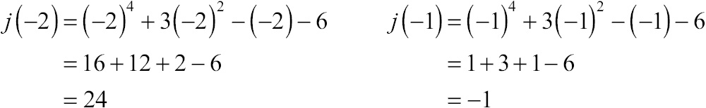
Function j(x) is continuous for its entire domain—there are no denominators that might equal zero and cause a vertical asymptote, no radical expressions that might be negative under a square root sign and become undefined, no piecewise-defined functions that might cause a break in the graph. All you have here is a nice, smooth, unbroken graph of a polynomial, and as long as the function is continuous over a closed domain, like [–2,–1], you can apply the Intermediate Value Theorem.
Watch carefully now. This problem is a lot like a magic trick—if you blink you might miss it. Here we go.
You know that the function j(x) passes through point (–2,24) and (–1,–1). According to the Intermediate Value Theorem, every y-value between 24 and –1 corresponds to some x-value between –2 and –1. That’s it—you’re done!
Did you miss it? Every y-value between 24 and –1, including 0, has a corresponding x-value between –2 and –1. In other words, at some x-value on the interval [–2,–1], y has a value of 0, causing a root or x-intercept in the graph.
Don’t get all muddled up in the semantics of the theorem. Here’s the gist of it. Imagine that there’s a huge line on the floor of the room you’re currently in, a line that divides the room roughly in half. Well, if at 10 A.M. you’re standing on one side of that line and at 11 A.M. you’re standing on the other side, then at some point between 10 and 11 A.M. (assuming you didn’t leave the room or teleport through space and time) you crossed the line.
If you are particularly interested, this happens at approximately x = –1.08, as you can see in the graph of j(x) in Figure 7.9.
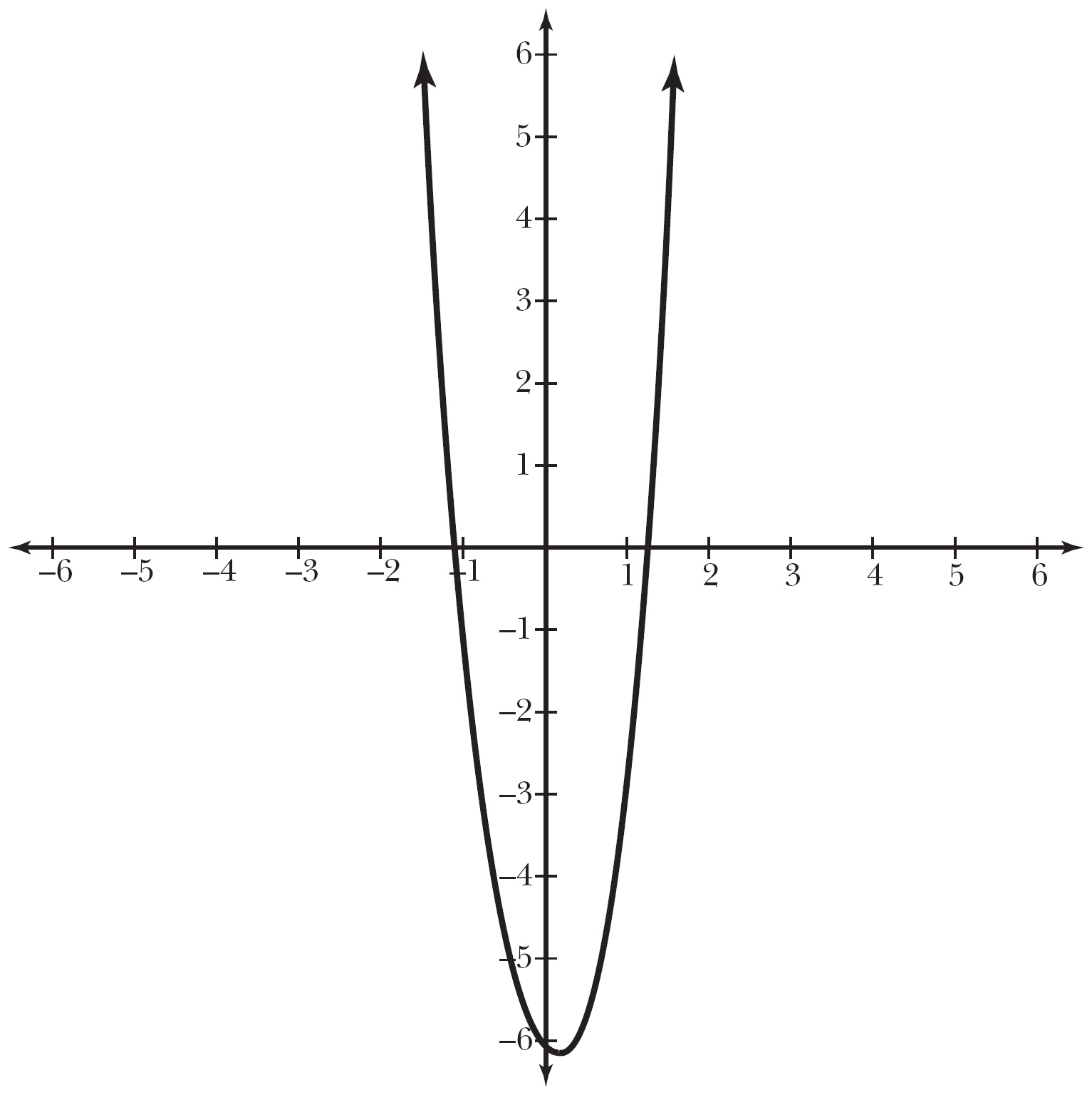
Figure 7.9
Function j(x) also has a root between x = 1 and x = 2.
You’ve got problems
Problem 4: Use the Intermediate Value Theorem to explain why the function g(x) = x2 + 3x – 6 must have a root on the interval [1,2].
The Least You Need to Know
- A continuous function has no holes, jumps, or breaks in its graph.
- If a function reaches its intended height at a particular x-value, the function is continuous there.
- If a function is undefined but possesses a limit at a given x-value, there is point discontinuity, which is removable.
- Infinite discontinuity is caused by a vertical asymptote, whereas jump discontinuity is caused by a break in the function’s graph; both are nonremovable discontinuities.
- The Intermediate Value Theorem uses rather complex language to guarantee the “wholeness” or “completeness” of a graph.