
Chi-Squared Tests for Specific Distributions
9.1 Tests for Poisson, binomial, and “binomial” approximation of Feller’s distribution
Let ![]() be independent and identically distributed random variables. Consider the problem of testing the composite hypothesis
be independent and identically distributed random variables. Consider the problem of testing the composite hypothesis ![]() according to which the distribution of
according to which the distribution of ![]() is a member of a parametric family with the Poisson distribution
is a member of a parametric family with the Poisson distribution
![]() (9.1)
(9.1)
Let ![]() be the observed frequencies meaning the number of realized values of
be the observed frequencies meaning the number of realized values of ![]() that fall into a specific class or interval
that fall into a specific class or interval ![]() , where the fixed integer grouping classes
, where the fixed integer grouping classes ![]() are such that
are such that ![]() . As before, let
. As before, let ![]() be a column vector of standardized grouped frequencies with its components as
be a column vector of standardized grouped frequencies with its components as
![]()
If the nuisance parameter ![]() is estimated effectively from grouped data by
is estimated effectively from grouped data by ![]() , then the standard Pearson’s sum
, then the standard Pearson’s sum ![]() will follow in the limit the chi-square distribution with
will follow in the limit the chi-square distribution with ![]() degrees of freedom. If, on the other hand, the parameter
degrees of freedom. If, on the other hand, the parameter ![]() is estimated from raw (ungrouped) data, for example, by the maximum likelihood estimate (MLE), then the standard Pearson test must be modified. Let
is estimated from raw (ungrouped) data, for example, by the maximum likelihood estimate (MLE), then the standard Pearson test must be modified. Let ![]() be a
be a ![]() (s being the dimensionality of the parameter space) matrix with its elements as
(s being the dimensionality of the parameter space) matrix with its elements as

For the null hypothesis in (9.1), the ![]() matrix
matrix ![]() possesses its elements as
possesses its elements as
![]()
Let ![]() be the MLE of
be the MLE of ![]() based on the raw data. Then, the well-known Nikulin-Rao–Robson (NRR) modified chi-squared test statistic, distributed in the limit as
based on the raw data. Then, the well-known Nikulin-Rao–Robson (NRR) modified chi-squared test statistic, distributed in the limit as ![]() , can be expressed as
, can be expressed as
![]() (9.2)
(9.2)
where ![]() and
and ![]() are the estimators of the Fisher information matrix (scalar) and of the column vector
are the estimators of the Fisher information matrix (scalar) and of the column vector ![]() , respectively.
, respectively.
Next, let us consider the binomial null hypothesis. Let the probability mass function be specified as
![]() (9.3)
(9.3)
where ![]() and
and ![]() . In this case, the Fisher information matrix (scalar) is
. In this case, the Fisher information matrix (scalar) is ![]() and the elements of the matrix
and the elements of the matrix ![]() are
are
![]()
Let ![]() be the MLE estimator of
be the MLE estimator of ![]() . Then, the modified chi-squared test statistic, distributed in the limit as
. Then, the modified chi-squared test statistic, distributed in the limit as ![]() , can be expressed as
, can be expressed as
![]() (9.4)
(9.4)
where ![]() and
and ![]() .
.
Now, let the probability distribution of the null hypothesis follow Feller’s 1948, pp. 105–115) discrete distribution with cumulative distribution function
 (9.5)
(9.5)
where ![]() is the complement gamma function.
is the complement gamma function.
If the parameter ![]() and
and ![]() , then the distribution function in (9.5) can be approximated as
, then the distribution function in (9.5) can be approximated as
![]()
Using the results of Bol’shev (1963) a more accurate approximation of (9.5) can be obtained as
![]() (9.6)
(9.6)
where ![]() and
and ![]() . Note that (9.6) looks like the binomial distribution function with the exception that the parameter
. Note that (9.6) looks like the binomial distribution function with the exception that the parameter ![]() can be any real positive number. Consider the probability mass function of (9.6) given by
can be any real positive number. Consider the probability mass function of (9.6) given by
![]() (9.7)
(9.7)
where the parameter ![]() . In this case, there are three possibilities to construct a modified chi-squared test for testing a composite null hypothesis about the distribution in (9.6). First one is to use MLEs of
. In this case, there are three possibilities to construct a modified chi-squared test for testing a composite null hypothesis about the distribution in (9.6). First one is to use MLEs of ![]() and
and ![]() and the NRR statistic
and the NRR statistic ![]() . Since the MLEs of
. Since the MLEs of ![]() and
and ![]() cannot be derived easily, the modified test
cannot be derived easily, the modified test ![]() based on MMEs (see Eq. (4.9)) or Singh’s
based on MMEs (see Eq. (4.9)) or Singh’s ![]() (see Eq. (3.25)) can be used.
(see Eq. (3.25)) can be used.
For the model in (9.7) and ![]() , the DN statistic
, the DN statistic ![]() will follow in the limit
will follow in the limit ![]() and
and ![]() . If
. If ![]() , then, as before (see Eq. (4.12)), we will have
, then, as before (see Eq. (4.12)), we will have

In this case, ![]() ,
, ![]() , and
, and
![]()
To specify the above tests, we of course will need explicit expressions of all the matrices involved.
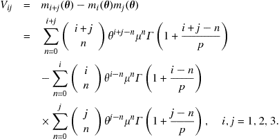
The elements of the Fisher information matrix ![]() for the model in (9.7) are
for the model in (9.7) are

where ![]() is the largest integer contained in
is the largest integer contained in ![]() and
and ![]() is the psi-function. It is known that series expansions for the psi-function converge very slowly. But, for integer values of x, a recurrence
is the psi-function. It is known that series expansions for the psi-function converge very slowly. But, for integer values of x, a recurrence ![]() can be used, from which it follows that
can be used, from which it follows that
![]()
This result permits us to calculate all expressions containing ![]() with a very high accuracy.
with a very high accuracy.
The elements of the matrix ![]() are
are

The elements of the matrix ![]() are
are
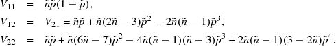
The elements of the matrix ![]() are
are

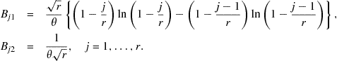
The components ![]() and
and ![]() of the vector
of the vector ![]() for Singh’s test
for Singh’s test ![]() for the model in (9.7) are
for the model in (9.7) are
![]()
and
![]()
It has to be noted that the test in (3.25) is computationally much more complicated than the statistic ![]() for large samples.
for large samples.
For the model in (9.7), ![]() and
and ![]() . Denoting the first two sample moments
. Denoting the first two sample moments ![]() and
and ![]() and then equating them to population moments, the MMEs of
and then equating them to population moments, the MMEs of ![]() and
and ![]() are obtained as
are obtained as
![]() (9.8)
(9.8)
From (9.8), we see that negative values of ![]() and
and ![]() are possible, but the proportion of such estimates will be almost negligible for samples of size
are possible, but the proportion of such estimates will be almost negligible for samples of size ![]() . It seems that
. It seems that ![]() test can be used for analyzing Rutherford’s data, but the question about
test can be used for analyzing Rutherford’s data, but the question about ![]() -consistency of the MMEs in (9.8) is still open.
-consistency of the MMEs in (9.8) is still open.
To examine the rate of convergence of estimators ![]() and
and ![]() for sample sizes
for sample sizes ![]() , we simulated 3,000 estimates of
, we simulated 3,000 estimates of ![]() and
and ![]() assuming that
assuming that ![]() and
and ![]() , values that correspond to Rutherford’s data. The power curve fit of
, values that correspond to Rutherford’s data. The power curve fit of ![]() , the average value of estimates
, the average value of estimates ![]() for 3000 runs, in Figure 9.1 shows that
for 3000 runs, in Figure 9.1 shows that ![]() and
and ![]() . The power curve fit of
. The power curve fit of ![]() in Figure 9.2 gives
in Figure 9.2 gives ![]() and
and ![]() . To check for the distribution of the statistic
. To check for the distribution of the statistic ![]() under the null “Feller’s” distribution (
under the null “Feller’s” distribution (![]() and
and ![]() ), we simulated
), we simulated ![]() values of
values of ![]() . The histogram of these values is well described by the
. The histogram of these values is well described by the ![]() distribution (see Figure 9.3). The average value
distribution (see Figure 9.3). The average value ![]() also does not contradict the assumption that the statistic
also does not contradict the assumption that the statistic ![]() follows in the limit the chi-squared distribution with one degree of freedom. Another important property of any test statistic is its independence from the unknown parameters. To check for this feature of the test
follows in the limit the chi-squared distribution with one degree of freedom. Another important property of any test statistic is its independence from the unknown parameters. To check for this feature of the test ![]() , we simulated
, we simulated ![]() values of
values of ![]() assuming that
assuming that ![]() (two times less than for the null hypothesis
(two times less than for the null hypothesis ![]() ) and
) and ![]() (two times more than for the null hypothesis
(two times more than for the null hypothesis ![]() ). The results (Figure 9.4) show that the simulated values do not contradict the independence, because the histogram is again well described by
). The results (Figure 9.4) show that the simulated values do not contradict the independence, because the histogram is again well described by ![]() distribution.
distribution.

Figure 9.1 Simulated average value of ![]() (circles) and the power function fit (solid line) as function of the sample size n.
(circles) and the power function fit (solid line) as function of the sample size n.

Figure 9.2 Simulated average value of ![]() (circles) and the power function fit (solid line) as function of the sample size n.
(circles) and the power function fit (solid line) as function of the sample size n.

Figure 9.3 The histogram of the 1000 simulated values of ![]() for the null hypothesis (
for the null hypothesis (![]() and
and ![]() ) and the
) and the ![]() distribution (solid line).
distribution (solid line).

Figure 9.4 The histogram of the 1000 simulated values of ![]() for
for ![]() and the
and the ![]() distribution (solid line).
distribution (solid line).
The above results evidently allow us to use the HRM statistic ![]() for Rutherford’s data analysis.
for Rutherford’s data analysis.
9.2 Elements of matrices K, B, C, and V for the three-parameter Weibull distribution
For r equiprobable cells of the model in (4.25), the borders of equiprobable intervals are defined as:
![]()
Then, the elements of the matrix ![]() are as follows:
are as follows:

where ![]() and
and ![]() is the psi-function. For the required calculation of
is the psi-function. For the required calculation of ![]() , we used the series expansion
, we used the series expansion
![]()
where ![]() is the Euler’s constant.
is the Euler’s constant.
Similarly, the elements of the matrices ![]() and
and ![]() are as follows:
are as follows:

where the population moments are

and ![]() is the incomplete gamma function. For the required calculation of
is the incomplete gamma function. For the required calculation of ![]() , we used the following series expansion (Prudnikov et al., 1981, p. 705):
, we used the following series expansion (Prudnikov et al., 1981, p. 705):
![]()
Finally, the elements of the matrix ![]() are as follows:
are as follows:
9.3 Elements of matrices J and B for the Generalized Power Weibull distribution
Elements ![]() of the Fisher information matrix
of the Fisher information matrix ![]() are as follows:
are as follows:

Next, the elements of matrix ![]() are as follows:
are as follows:

9.4 Elements of matrices J and B for the two-parameter exponential distribution
Consider the two-parameter exponential distribution with cumulative distribution function
![]() (9.9)
(9.9)
where the unknown parameter ![]() . It is easily verified that the matrix
. It is easily verified that the matrix ![]() for the model in (9.9) is
for the model in (9.9) is
 (9.10)
Based on the set of n i.i.d. random variables ![]() , the MLE
, the MLE ![]() of the parameter
of the parameter ![]() equals
equals ![]() , where
, where
![]() (9.11)
(9.11)
Consider r disjoint equiprobable intervals
![]()
For these intervals, the elements of the matrix ![]() (see Eq. (3.4)) are
(see Eq. (3.4)) are
Using the matrix in (9.10) and the above elements of the matrix ![]() with
with ![]() replaced by the MLE
replaced by the MLE ![]() in (9.11), the NRR test
in (9.11), the NRR test ![]() (see Eq. (3.8)) can be used. While using Microsoft Excel, the calculations based on double precision is recommended.
(see Eq. (3.8)) can be used. While using Microsoft Excel, the calculations based on double precision is recommended.
9.5 Elements of matrices B, C, K, and V to test the logistic distribution
Let ![]() , and
, and ![]() , be borders of r equiprobable random grouping intervals. Then, the probabilities of falling into each interval are
, be borders of r equiprobable random grouping intervals. Then, the probabilities of falling into each interval are ![]() .
.
The elements of the ![]() matrix
matrix ![]() , for
, for ![]() , are as follows:
, are as follows:

Next, the elements of the ![]() matrix
matrix ![]() are as follows:
are as follows:

where ![]() is Euler’s dilogarithm function that can be computed by the series expansion
is Euler’s dilogarithm function that can be computed by the series expansion
![]()
and by the expansion
![]()
for ![]() (Prudnikov et al., 1986, p. 763).
(Prudnikov et al., 1986, p. 763).
Finally, we have the matrices ![]() and
and ![]() as
as
![]()
9.6 Testing for normality
System requirements for implementing the software of Sections 9.6, 9.7, 9.8, 9.9, 9.10 are Windows XP, Windows 7, MS Office 2003, 2007, 2010.
1. Open file Testing Normality.xls;
2. Enter your sample data in column “I” starting from cell 1;
3. Click the button “Compute,” introduce the sample size and the desired number of equiprobable intervals ![]() . The recommended number of intervals for the NRR test
. The recommended number of intervals for the NRR test ![]() in (3.8), under close alternatives (such as the logistic), is
in (3.8), under close alternatives (such as the logistic), is ![]() . The recommended number of intervals for the test
. The recommended number of intervals for the test ![]() in (3.24) is
in (3.24) is ![]() (see Section 4.4.1). Note that the power of
(see Section 4.4.1). Note that the power of ![]() can be more than that of the NRR test;
can be more than that of the NRR test;
5. Numerical values of ![]() and
and ![]() are in cells F2 and G2, respectively. Cells F3 and G3 contain the corresponding percentage points at level 0.05. The P-values of
are in cells F2 and G2, respectively. Cells F3 and G3 contain the corresponding percentage points at level 0.05. The P-values of ![]() and
and ![]() are in cells F4 and G4, respectively.
are in cells F4 and G4, respectively.
9.7 Testing for exponentiality
9.7.1 Test of Greenwood and Nikulin (see Section 3.6.1)
1. Open file Testing Exp GrNik.xls;
2. Enter your sample data in column “I” starting from cell 1;
3. Click the button “Compute,” introduce the sample size and desired number of equiprobable intervals. The recommended number of equiprobable intervals is ![]() ;
;
5. The numerical value of ![]() (see Eq. (3.44)) is in cell F2. The percentage point at level 0.05 and the P-value are in cells F3 and F4, respectively.
(see Eq. (3.44)) is in cell F2. The percentage point at level 0.05 and the P-value are in cells F3 and F4, respectively.
9.7.2 Nikulin-Rao-Robson test (see Eq. (3.8) and Section 9.4)
1. Open file Testing NRR 2-param EXP.xls;
2. Enter your sample data in column “I” starting from cell 1;
3. Click the button “Compute,” introduce the sample size and desired number of equiprobable intervals. The recommended number of equiprobable intervals is ![]() ;
;
5. The numerical value of ![]() is in cell F2. The percentage point at level 0.05 and the P-value are in cells F3 and F4, respectively.
is in cell F2. The percentage point at level 0.05 and the P-value are in cells F3 and F4, respectively.
9.8 Testing for the logistic
1. Open file Testing Logistic.xls;
2. Enter your sample data in column “I” starting from cell 1;
3. Click the button “Compute,” introduce the sample size and desired number of equiprobable intervals ![]() . The recommended number of equiprobable intervals, for close alternatives (such as normal), is
. The recommended number of equiprobable intervals, for close alternatives (such as normal), is ![]() ;
;
5. Numerical values of ![]() in (4.9) and
in (4.9) and ![]() in (4.13) are in cells E2 and F2, respectively. Cells E3 and F3 contain the corresponding percentage points at level 0.05. The P-values of
in (4.13) are in cells E2 and F2, respectively. Cells E3 and F3 contain the corresponding percentage points at level 0.05. The P-values of ![]() and
and ![]() are in cells E4 and F4, respectively.
are in cells E4 and F4, respectively.
9.9 Testing for the three-parameter Weibull
1. Open file Testing Weibull3.xls;
2. Enter your sample data in column “I” starting from cell 1;
3. Click the button “Compute,” introduce the sample size and desired number of equiprobable intervals ![]() . The recommended number of equiprobable intervals for the Exponentiated Weibull and Power Generalized Weibull alternatives is
. The recommended number of equiprobable intervals for the Exponentiated Weibull and Power Generalized Weibull alternatives is ![]() ;
;
5. Numerical values of ![]() in (4.9) and
in (4.9) and ![]() in (4.14) (see also Section 9.2) are in cells F2 and G2, respectively. Note that the power of
in (4.14) (see also Section 9.2) are in cells F2 and G2, respectively. Note that the power of ![]() is usually higher than that of
is usually higher than that of ![]() . Cells F3 and G3 contain the corresponding percentage points at level 0.05. The P-values of
. Cells F3 and G3 contain the corresponding percentage points at level 0.05. The P-values of ![]() and
and ![]() are in cells F4 and G4, respectively.
are in cells F4 and G4, respectively.
9.10 Testing for the Power Generalized Weibull
1. Open file Test for PGW (Left-tailed).xls;
2. Enter your sample data in column “I” starting from cell 1;
3. Click the button “Run,” introduce the sample size and desired number of equiprobable intervals ![]() . The recommended number of equiprobable intervals for the Exponentiated Weibull, Generalized Weibull, and Three-Parameter Weibull alternatives is
. The recommended number of equiprobable intervals for the Exponentiated Weibull, Generalized Weibull, and Three-Parameter Weibull alternatives is ![]() ;
;
4. Click OK. Note that the power of ![]() in (3.50) is usually higher than that of
in (3.50) is usually higher than that of ![]() in (3.48);
in (3.48);
5. Numerical values of ![]() and
and ![]() (see Eqs. (3.48), (3.50) and Section 9.3) are in cells F2 and G2, respectively. Cells F3 and G3 contain the corresponding percentage points at level 0.05. The P-values of
(see Eqs. (3.48), (3.50) and Section 9.3) are in cells F2 and G2, respectively. Cells F3 and G3 contain the corresponding percentage points at level 0.05. The P-values of ![]() and
and ![]() are in cells F4 and G4, respectively.
are in cells F4 and G4, respectively.
9.11 Testing for two-dimensional circular normality
1. Open file Testing Circular Normality.xls;
2. Enter your sample data in columns “I” and “J” starting from cell 1;
3. Click the button “Compute,” introduce the sample size and the desired number of equiprobable intervals. The recommended number of intervals for the two-dimensional logistic alternative is ![]() , while the recommended number of intervals for the two-dimensional normal alternative is 3;
, while the recommended number of intervals for the two-dimensional normal alternative is 3;
5. Numerical values of ![]() and
and ![]() (see Section 3.5.3) are in cells F2 and G2, respectively. Cells F3 and G3 contain the corresponding percentage points at level 0.05. The P-values of
(see Section 3.5.3) are in cells F2 and G2, respectively. Cells F3 and G3 contain the corresponding percentage points at level 0.05. The P-values of ![]() and
and ![]() are in cells F4 and G4, respectively.
are in cells F4 and G4, respectively.
References
1. Bol’shev LN. Asymptotical Pearson’s transformations. Theory of Probability and its Applications. 1963;8:129–155.
2. Feller W. On probability problems in the theory of counters. In: Courant Anniversary Volume. New York: Interscience Publishers; 1948;105–115.
3. Prudnikov AP, Brychkov YA, Marichev OI. Integrals and Series. Nauka, Moscow: Elementary Functions; 1981.
4. Prudnikov AP, Brychkov YA, Marichev OI. Integrals and Series. Nauka, Moscow: Additional Chapters; 1986.