Characterizing Relative Costs and Workload Variability

To decide which approach to use, we need to characterize a few main parameters. The first is the unit cost of an on-demand, pay-per-use cloud resource relative to the unit cost of a dedicated resource, which may be owned and incur a cost for depreciation, may be leased and incur a monthly fee, or may be financed, and represent an ongoing principal plus interest fee to the bank. We will define a “utility premium,” U, as the ratio of the cloud unit cost to the do-it-yourself unit cost. In an example where an owned car costs $10/day and a rental costs $50/day, the premium for the rental car is U = 5, since the rental car costs five times as much.

If U = 1, the cloud costs the same as ownership. It is like getting the rental car for $10 per day. And if U < 1, the cloud is cheaper, which certainly can happen as well. The utility premium, U, may vary over time, due both to improvements or one-time charges in your own operations and to price reductions or increases that the cloud provider may implement. However, here we adopt the convenient fiction that U is constant. We assume that the cost of the “ownership” model for a resource for a unit time is cr and therefore that the cost of the utility pricing in the cloud is U × cr. For a given amount of time, T, the total price incurred for an owned resource is cr × T, and the total price for that in the cloud is U × cr × T. These formulas are just a way of formalizing what we’ve already discussed. In the rental car case where the fee for three days was $150, we had U = 5, that is, the rental cost five times as much as owned car; cr = $10 per day; and T = 3 days.

The other characteristic that we want to consider is the degree of variability of demand. Normally, statisticians use measures such as variance and standard deviation. For now, we use a much simpler characterization: peak, P, and average, A, which we can combine into a peak-to-average ratio: P/A. Exhibit 11.1 illustrates a typical variable demand for a Web site, an internal application—or it could be electricity utilization or automobile purchases or anything. As can be seen, over this time horizon, there is a peak and an average.

EXHIBIT 11.1 Variable Demand and Peak and Average Metrics

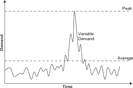
You may remember from Chapter 8 that Google’s demand over a several-month period was almost as flat as a midwestern plain. Its peak was basically its average (i.e., P≅A). However, the retailers tended to have a mountain beginning around Thanksgiving, which rises from the mesa that is their everyday demand. The baseline demand is not the average but in most cases will be relatively close, because if we were to “bulldoze” the mountain and spread the rubble around, it wouldn’t raise the surface of the mesa by very much. A good example of a ratio of a medium-size peak to average is Walmart.com from Chapter 8, with an approximate average of .025% of daily page views, and a peak of .16% of daily page views, for a P/A of 6.4.

Then there are the really high peak-to-average workloads, such as the spike in telephony traffic that the Sonus Networks data in Chapter 8 showed on New Year’s Eve. The Olympics Web sites are another example, with large numbers of visitors for two weeks every couple of years but much less the rest of the time. One thing to note is that the peak must always be greater than or equal to the average. When the peak equals the average, demand is perfectly flat.

Armed with only this information, we can make a number of intelligent decisions. In Chapter 9 we discussed the optimal resourcing strategy for a simple case of uniformly distributed demand, which is partly dependent on the nature of the workload and partly dependent on the relative penalties associated with excess resources versus unmet demand. Of course, there are other demand distributions as well, such as normally distributed (bell curve) demand. We assume that a better-safe-than-sorry strategy is deployed, such that an enterprise has enough dedicated resources to meet its peak demand.

Given all this, if an enterprise has resources that are built to peak, P, for a given amount of time, T, the enterprise cost is simply P × cr × T. With the pay-per-use strategy of the cloud, the price each day, or hour, or minute may vary, and this may seem like a challenge to model. However, the average encodes the impact of this variation. Having one rental car for one day and then three rental cars the next day costs no more or less than having two cars—the average quantity—for the two days. Either way costs four rental days (we are ignoring volume discounts, getting the fifth day free, or other promotions and deals).

Consequently, the cloud cost is just the average quantity of resources used times the cloud price, which is the base resource cost times the utility premium, times the duration for which those costs were incurred: A × U × cr × T.

Armed with nothing more than these two equations for enterprise cost and cloud cost, we can draw some important conclusions.