
Chapter 4. CockroachDB SQL
The language of CockroachDB is SQL. While there are some command-line utilities, all interactions between an application and the database are mediated by SQL language commands.
SQL is a rich language with a long history – we touched upon some of that history in Chapter 1. A full definition of all SQL language features would require a book in its own right and would be almost instantly out of date since the SQL language evolves with each release.
Therefore, this chapter aims to provide you with a broad overview of the SQL language used in CockroachDB without attempting to be a complete reference. We’ll take a task-oriented approach to the SQL language, covering the most common SQL language tasks with particular reference to unique features of the CockroachDB SQL implementation.
A complete reference for the CockroachDB SQL language can be found in the CockroachDB documentation set1. A broader review of the SQL language can be found in the O’Reilly book “SQL in a Nutshell”.
We’ll mainly use the MOVR sample dataset in this chapter to illustrate various SQL language features. We learned how to install sample data in Chapter 2; to recap, we create the MOVR database by issuing the command + cockroach workload init movr+ command:
$cockroach workload init movr I210510 01:311imported users(0s,50rows)I210510 01:312imported vehicles(0s,15rows)I210510 01:313imported rides(0s,500rows)I210510 01:314imported vehicle_location_histories(0s,1000rows)I210510 01:315imported promo_codes(0s,1000rows)I210510 01:3116starting8splits I210510 01:3117starting8splits I210510 01:3118starting8splits
You may also wish to run the command cockroach workload run movr to generate ride data against the MOVR base tables.
SQL LANGUAGE COMPATIBILITY
CockroachDB is broadly compatible with the PostgreSQL implementation of the SQL:2016 standard. The SQL:2016 standard contains a number of independent modules, and no major database implements all of the standards. However, the PostgreSQL implementation of SQL is arguably as close to “standard” as exists in the database community.
CockroachDB varies from PostgreSQL in a couple of areas:
-
CockroachDB does not currently support stored procedures, events or triggers. In PostgreSQL, these stored procedures allow for the execution of program logic within the database server, either on-demand or in response to some triggering event.
-
CockroachDB does not currently support User Defined Functions
-
CockroachDB does not support PostgreSQL XML functions.
-
CockroachDB does not support PostgreSQL FullText indexes and functions.
QUERYING DATA WITH SELECT
Although we need to create and populate tables before querying them, it is logical to start with the SELECT statement since many features of the SELECT statement appear in other types of SQL – subqueries in UPDATEs for instance – and for data scientists and analysts, the SELECT statement is often the only SQL statement they ever need to learn.
The SELECT statement (Figure 4-1) is the workhorse of relational query and has a complex and rich syntax. The CockroachDB SELECT statement implements the standard features of the standard SELECT, with just a few CockroachDB-specific features.
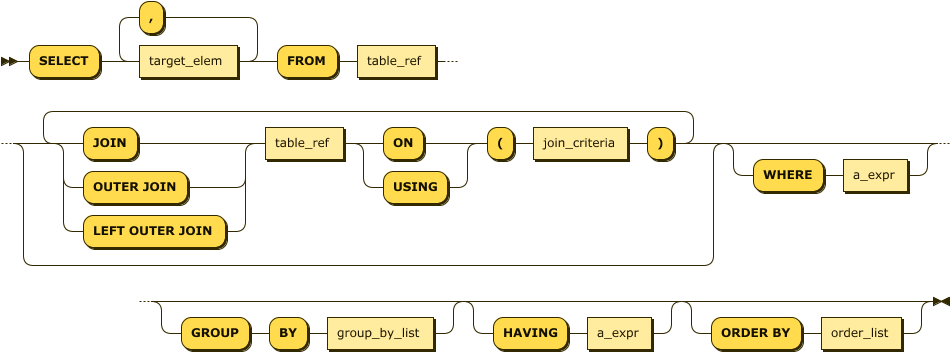
Figure 4-1. Select Statement
In the following sections, we’ll examine each of the major elements of the SELECT statement as well as the functions and operators that can be included in a SELECT statement.
The SELECT list
A very simple SQL statement consists of nothing but a SELECT statement together with scalar expressions. For instance:
SELECTCONCAT('Hello from CockroachDB at ',CAST(NOW()asSTRING))ashello
The SELECT list includes a comma-separated list of expressions that can contain combinations of constants, functions, and operators. The CockroachDB SQL language supports all the familiar SQL operators. A complete list of functions and operators can be found in the CockroachDB documentation set2.
The FROM clause
The FROM clause is the primary method of attaching table data to the SELECT statement. In its most simple incarnation, all rows and columns from a table can be fetched:
SELECT*FROMrides
Table names may be aliased using the AS clause or simply by following the table name with an alias. That alias can then be used anywhere in the query to refer to the table. Column names can also be aliased. For instance, the following are all equivalent:
SELECTnameFROMusers;SELECTu.nameFROMusersu;SELECTusers.nameFROMusersu;SELECTusers.nameASuser_nameFROMusers;SELECTu.nameFROMusersASu;
JOINS
Joins allow the results from two or more tables to be merged based on some common column values.
The inner join is the default join operation. In this join, rows from one table are joined to rows from another table based on some common (“key”) values. Rows that have no match in both tables are not included in the results. For instance, the following query links vehicle and ride information in the MOVR database:
SELECTv.id,v.ext,r.start_timer.start_addressFROMvehiclesvLEFTOUTERJOINridesrON(r.vehicle_id=v.id);
Note that a vehicle that had not been involved in a ride would not be included in the result set.
The ON clause specifies the conditions which join the two tables – in the above query, the columns vehicle_id in the rider table were matched with the id column in the vehicles table. If the join is on an identically named column in both tables, then the USING clause provides a handy shortcut. Here we join users and user_ride_counts using the common name column:
SELECT*FROMusersuJOINuser_ride_countsurcUSING(name)
The Outer join allows rows to be included even if they have no match in the other table. Rows that are not found in the outer join table are represented by NULL values. LEFT and RIGHT determine which table may have missing values. For instance, the following query prints all the users in the users table, even if some are not associated with a promo code:
SELECTu.name,upc.codeFROMUSERSuLEFTOUTERJOINuser_promo_codesupcON(u.id=upc.user_id);
The RIGHT anti-join reverses the outer join. So, this query is identical to the previous query since the users table is now the “right” table in the join:
SELECTDISTINCTu.name,upc.codeFROMuser_promo_codesupcRIGHTOUTERJOINUSERSuON(u.id=upc.user_id);
Anti-joins
It is often required to select all rows from a table that do not have a matching row in some other result set. This is called an anti-join, and while there is no SQL syntax for this concept, it is typically implemented using a subquery and the IN or EXISTS clause. The query planner recognizes this pattern and executes the query using a version of the JOIN machinery. The following examples illustrate the anti-join using the EXISTS and IN operators.
Each example selects employees who are not also customers.
SELECT*FROMusersWHEREidNOTIN(SELECTidFROMemployees)
This query returns the same results but using a correlated sub-query (we’ll discuss subqueries in more detail in an upcoming section):
SELECT*FROMusersuWHERENOTEXISTS(SELECTidFROMemployeeseWHEREe.id=u.id)
CROSS JOINS
CROSS JOIN indicates that every row in the left table should be joined to every row in the right table. Usually, this is a recipe for disaster unless one of the tables has only one row or is a laterally correlated subquery (see the section on correlated subqueries later in this chapter).
Set operations
SQL implements a number of operations that deal directly with result sets. These operations collectively referred to as “set operations” allow result sets to be concatenated, subtracted, or overlaid.
The most common of these operations is the UNION operator, which returns the sum of two result sets. By default, duplicates in each result set are eliminated. By contrast, the UNION ALL operation will return the sum of the two result sets, including any duplicates. The following example returns a list of customers and employees. Employees who are also customers will only be listed once:
SELECTname,addressFROMcustomersUNIONSELECTname,addressFROMemployees;
INTERSECT returns those rows which are in both result sets. This query returns customers who are also employees:
SELECTname,addressFROMcustomersINTERSECTSELECTname,addressFROMemployees;
EXCEPT returns rows in the first result set which are not present in the second. This query returns customers who are not also employees:
SELECTname,addressFROMcustomersEXCEPTSELECTname,addressFROMemployees;
All set operations require that the component queries return the same number of columns and that those columns are of a compatible data type.
Group operations
Aggregate operations allow for summary information to be generated, typically upon groupings of rows. Rows can be grouped using the GROUP BY operator. If this is done, the select list must consist only of columns contained within the GROUP BY clause and aggregate functions.
The most common aggregate functions are shown in Table 4-1.
AVG |
Calculate the average value for the group. |
COUNT |
Return the number of rows in the group. |
MAX |
Return the maximum value in the group. |
MIN |
Return the minimum value in the group. |
STDDEV |
Return the standard deviation for the group. |
SUM |
-Return the total of all values for the group. |
The following example generates summary ride information for each city:
SELECTu.city,SUM(urc.rides),AVG(urc.rides),max(urc.rides)FROMusersuJOINuser_ride_countsurcUSING(name)GROUPBYu.city
Subqueries
A subquery is a SELECT statement that occurs within another SQL statement. Such a “nested” SELECT statement can be used in a wide variety of SQL contexts, including SELECT, DELETE, UPDATE, and INSERT statements.
The following statement uses a subquery to count the number of rides that share the maximum ride length:
SELECTCOUNT(*)FROMridesWHERE(end_time-start_time)=(SELECTMAX(end_time-start_time)FROMrides);
Subqueries may also be used in the FROM clause wherever a table or view definition could appear. This query generates a result which compares each ride with the average ride duration for the city:
SELECTid,city,(end_time-start_time)ride_duration,avg_ride_durationFROMridesJOIN(SELECTcity,AVG(end_time-start_time)avg_ride_durationFROMridesGROUPBYcity)USING(city);
Correlated subquery
A correlated subquery is one in which the subquery refers to values in the parent query or operation. The subquery returns a potentially different result for each row in the parent result set. We saw an example of a correlated sub-query when performing an “anti-join” earlier in the chapter.
SELECT*FROMusersuWHERENOTEXISTS(SELECTidFROMemployeeseWHEREe.id=u.id)
Subqueries can often be used to perform an operation that is functionally equivalent to a join. In many cases, the query optimizer will transform these statements to joins so as to streamline the optimization process.
Lateral subquery
When a subquery is used in a join, the LATERAL keyword indicates that the subquery may access columns generated in preceding FROM table expressions. For instance, in the following query, the LATERAL keyword allows the subquery to access columns from the USERS table:
SELECTname,address,start_timeFROMUSERSCROSSJOINLATERAL(SELECT*FROMridesWHERErides.start_address=users.address)r;
This example is a bit contrived, and clearly, we could construct a simple join that performed this query more naturally. Where LATERAL joins really shine is in allowing subqueries to access computed columns in other subqueries within a FROM clause. See the CockroachDB documentation3 for a more serious example of lateral subqueries.
The WHERE clause
The WHERE clause is common to SELECT, UPDATE, and DELETE statements. It specifies a set of logical conditions that must evaluate to TRUE for all rows to be returned or processed by the SQL statement concerned.
Common Table expressions
SQL statements with a lot of subqueries can be hard to read and maintain, especially if the same subquery is needed in multiple contexts within the query. For this reason, SQL supports Common Table Expressions using the WITH clause. Figure 4-2 shows the syntax of a Common Table Expression.

Figure 4-2. Common Table Expression
In its simplest form, a Common Table Expression is simply a named query block that can be applied wherever a table expression can be used. For instance, here we create a Common Table Expression riderRevenue with the WITH clause, then refer to it in the FROM clause of the main query:
WITHriderRevenueAS(SELECTu.id,SUM(r.revenue)ASsumRevenueFROMridesrJOIN"users"uON(r.rider_id=u.id)GROUPBYu.id)SELECT*FROM"users"u2JOINriderRevenuerrUSING(id)ORDERBYsumrevenueDESC
The RECURSIVE clause allows the Common Table Expression to refer to itself, potentially allowing for a query to return an arbitrarily high (or even infinite) set of results. For instance, if the employees table contained a manager_id column which referred to the ‘manager’s row in the same table, then we could print a hierarchy of employees and managers as follows:
WITHRECURSIVEemployeeMgrAS(SELECTid,manager_id,name,NULLASmanager_name,1ASlevelFROMemployeesmanagersWHEREmanager_idISNULLUNIONALLSELECTsubordinates.id,subordinates.manager_id,subordinates.name,managers.name,managers.LEVEL+1FROMemployeeMgrmanagersJOINemployeessubordinatesON(subordinates.manager_id=managers.id))SELECT*FROMemployeeMgr
The MATERIALIZED clause forces CockroachDB to store the results of the Common Table Expression as a temporary table rather than re-executing it on each occurrence. This can be useful if the Common Table Expression is referenced multiple times in the query.
ORDER BY
The ORDER BY clause allows query results to be returned in sorted order. Figure 4-3 shows the ORDER BY syntax.

Figure 4-3. Order By
In the simplest form, ORDER BY takes one or more column expressions or column numbers from the SELECT list.
In this example, we sort by column numbers:
SELECTcity,start_time,(end_time-start_time)durationFROMridesrORDERBY1,3DESC
And in this case by column expressions:
SELECTcity,start_time,(end_time-start_time)durationFROMridesrORDERBYcity,(end_time-start_time)DESC
You can also order by an index. In the following example, rows will be ordered by city and start_time, since those are the columns specified in the index:
CREATEINDEXrides_start_timeONrides(city,start_time);SELECTcity,start_time,(end_time-start_time)durationFROMridesORDERBYINDEXrides@rides_start_time;
The use of ORDER BY INDEX guarantees that the index will be used to directly return rows in sorted order, rather than having to perform a sort operation on the rows after they are retrieved. See Chapter 8 for more advice on optimizing statements that contain an ORDER BY.
Window functions
Window functions are functions that operate over a subset – a “window” of the complete set of the results. Figure 4-4 shows the syntax of a Window function.

Figure 4-4. Window Function Syntax
PARTITION BY and ORDER BY create a sort of “virtual table” that the function works with. For instance, this query lists the top ten rides in terms of revenue, with the percentage of the total revenue and city revenue displayed:
SELECTcity,r.start_time,revenue,revenue*100/SUM(revenue)OVER()ASpct_total_revenue,revenue*100/SUM(revenue)OVER(PARTITIONBYcity)ASpct_city_revenueFROMridesrORDERBY5DESCLIMIT10
There are some aggregation functions that are specific to Windowing functions. RANK() ranks the existing row within the relevant window, and DENSE_RANK() does the same while allowing no “missing” ranks. LEAD and LAG provide access to functions in adjacent partitions.
For instance, this query returns the top 10 rides, with each ‘ride’s overall rank and rank within the city displayed:
SELECTcity,r.start_time,revenue,RANK()OVER(ORDERBYrevenueDESC)AStotal_revenue_rank,RANK()OVER(PARTITIONBYcityORDERBYrevenueDESC)AScity_revenue_rankFROMridesrORDERBYrevenueDESCLIMIT10;
Other SELECT clauses
The LIMIT clause limits the number of rows returned by a SELECT while the OFFSET clause “jumps ahead” a certain number of rows. This can be handy to paginate through a result set though it is almost always more efficient to use a filter condition to navigate to the next subset of results since otherwise, each request will need to reread and discard an increasing number of rows.
CockroachDB arrays
The ARRAY type allows a column to be defined as a one-dimensional array of elements, each of which shares a common data type. We’ll talk about arrays in the context of data modeling in the next chapter. Although they can be useful, they are strictly speaking a violation of the relational model and should be used carefully.
An ARRAY variable is defined by adding “[]” or the word “ARRAY” to the datatype of a column. For instance:
CREATETABLEa(bSTRING[]);CREATETABLEc(dINTARRAY);
The ARRAY function allows us to insert multiple items into the ARRAY:
INSERTINTOaVALUES(ARRAY['sky','road','car']);SELECT*FROMa;b------------------{sky,road,car}
We can access an individual element of an array with the familiar array element notation:
SELECTarrayColumn[2]FROMarrayTable;arraycolumn---------------Road
The “@>” operator can be used to find arrays that contain one or more elements:
SELECT*FROMarrayTableWHEREarrayColumn@>ARRAY['road'];arraycolumn------------------{sky,road,car}
We can add elements to an existing array using the ARRAY_APPEND function and remove elements using ARRAY_REMOVE.
UPDATEarrayTableSETarrayColumn=array_append(arrayColumn,'cat')WHEREarrayColumn@>ARRAY['car']RETURNINGarrayColumn;arraycolumn----------------------{sky,road,car,cat}UPDATEarrayTableSETarrayColumn=array_remove(arrayColumn,'car')WHEREarrayColumn@>ARRAY['car']RETURNINGarrayColumn;arraycolumn------------------{sky,road,cat}
Finally, the UNNEST function transforms an array into a tabular result – one row for each element of the array. This can be used to “join” the contents of an array with data held in relational form elsewhere in the database. We show an example of this in the next chapter:
SELECTunnest(arrayColumn)FROMarrayTable;unnest----------skyroadcat
Working with JSON
The JSONB data type allows us to store JSON documents into a column, and CockroachDB provides operators and functions to help us work with JSON.
For these examples, we’ve created a table with a primary key CUSTOMERID and all data in a JSONB column JSONDATA. We can use the jsonb_pretty function to retrieve the JSON in a nicely formatted manner:
root@:26257/json>SELECTjsonb_pretty(jsondata)FROMcustomersjsonWHEREcustomerid=1;jsonb_pretty------------------------------------------------------{"Address":"1913 Hanoi Way","City":"Sasebo","Country":"Japan","District":"Nagasaki","FirstName":"MARY","LastName":"Smith","Phone":886780309,"_id":"5a0518aa5a4e1c8bf9a53761","dateOfBirth":"1982-02-20T13:00:00.000Z","dob":"1982-02-20T13:00:00.000Z","randValue":0.47025846594884335,"views":[{"filmId":611,"title":"MUSKETEERS WAIT","viewDate":"2013-03-02T05:26:17.645Z"},{"filmId":308,"title":"FERRIS MOTHER","viewDate":"2015-07-05T20:06:58.891Z"},{"filmId":159,"title":"CLOSER BANG","viewDate":"2012-08-04T19:31:51.698Z"},/* Some data removed */]}
Each JSON document contains some top-level attributes and a nested array of documents that contains details of films that they have streamed.
We can reference specific JSON attributes in the SELECT clause using the “->” operator:
root@:26257/json>SELECTjsondata->'City'ASCityFROMcustomersjsonWHEREcustomerid=1;city------------"Sasebo"
The “->>” operator is similar but returns the data formatted as text, not JSON.
If we want to search inside a JSONB column, we can use the “@>” operator:
SELECTCOUNT(*)FROMcustomersjsonWHEREjsondata@>'{"City": "London"}';count---------3
We often get the same result using the “->>” operator:
SELECTCOUNT(*)FROMcustomersjsonWHEREjsondata->>'City'='London';count---------3
We can interrogate the structure of the JSON document using the JSONB_EACH and JSONB_OBJECT_KEYS functions. JSONB_EACH returns one row per attribute in the JSON document, while JSONB_OBJECT_KEYS returns just the attribute keys. This is useful if you don’t know what is stored inside the JSONB column.
JSONB_ARRAY_ELEMENTS returns one row for each element in a JSON array. For instance, here we expand out the VIEWS array for a specific customer, counting the number of movies that they have seen:
SELECTCOUNT(jsonb_array_elements(jsondata->'views'))FROMcustomersjsonWHEREcustomerid=1;count---------37(1row)
Summary of SELECT
The SELECT statement is probably the most widely used statement in database programming and offers a very wide range of functionality. Even after decades of working in the field, the three of us don’t know every nuance of SELECT functionality. However, here we’ve tried to provide you with the most important aspects of the language. For more depth, view the CockroachDB documentation set4.
Although some database professionals use SELECT almost exclusively, the majority will be creating and manipulating data as well. In the following sections, we’ll look at the language features that support those activities.
CREATING TABLES AND INDEXES
In a relational database, data can only be added to pre-defined tables. These tables are created by the CREATE TABLE statement. Indexes can be created to enforce unique constraints or to provide a fast access path to the data. Indexes can be defined within the CREATE TABLE statement or by a separate CREATE INDEX statement.
The structure of a database schema forms a critical constraint on database performance and also on the maintainability and utility of the database. We’ll discuss the key considerations for database design in Chapter 5. For now, let’s create a few simple tables.
We use CREATE TABLE to create a table within a database. Figure 4-5 provides a simplified syntax for the CREATE TABLE statement.

Figure 4-5. Create Table Statement
A very simple CREATE TABLE is shown below. It creates a table mytable with a single column mycolumn. The mycolumn column can store only integer values.
CREATETABLEmytable(mycolumnint)
The CREATE TABLE statement must define the columns that occur within the table and can optionally define indexes, column families, constraints, and partitions associated with the table. For instance, the CREATE TABLE statement for the rides table in the movr database would look something like this:
CREATETABLEpublic.rides(idUUIDNOTNULL,cityVARCHARNOTNULL,vehicle_cityVARCHARNULL,rider_idUUIDNULL,vehicle_idUUIDNULL,start_addressVARCHARNULL,end_addressVARCHARNULL,start_timeTIMESTAMPNULL,end_timeTIMESTAMPNULL,revenueDECIMAL(10,2)NULL,CONSTRAINT"primary"PRIMARYKEY(cityASC,idASC),CONSTRAINTfk_city_ref_usersFOREIGNKEY(city,rider_id)REFERENCESpublic.users(city,id),CONSTRAINTfk_vehicle_city_ref_vehiclesFOREIGNKEY(vehicle_city,vehicle_id)REFERENCESpublic.vehicles(city,id),INDEXrides_auto_index_fk_city_ref_users(cityASC,rider_idASC),INDEXrides_auto_index_fk_vehicle_city_ref_vehiclesvehicle_cityASC,vehicle_idASC),CONSTRAINTcheck_vehicle_city_cityCHECK(vehicle_city=city));
This CREATE TABLE statement specified additional columns, their nullability, primary and foreign keys, indexes, and constraints upon table values.
The relevent clauses in Figure 4-5 are listed in Table 4-2.
column_def |
The definition of a column. This includes the column name, datatype, and nullability. Constraints specific to the column can also be included here, though it’s better practice to list all constraints separately. |
Index_def |
Definition of an index to be created on the table. Same as CREATE INDEX but without the leading |
table_contraint |
A constraint on the table, such as PRIMARY KEY, FOREIGN KEY, or CHECK. See below for constraint syntax. |
family_def |
Assigns columns to a column family. See Chapter 2 for more information about column families. |
Let’s now look at each of these CREATE TABLE options.
Column Definitions
A column definition consists of a column name, datatype, nullability status, default value, and possibly column-level constraint definitions. At a minimum, the name and data type must be specified. Figure 4-6 shows the syntax for a column definition.

Figure 4-6. Column Definition
Although constraints may be specified directly against column definitions, they may also be independently listed below the column definitions. Many practitioners prefer to list the constraints separately in this manner because it allows all constraints, including multi-column constraints, to be located together.
Computed Columns
CockroachDB allows tables to include computed columns that in some other databases would require a view definition.
column_nameASexpression[STORED|VIRTUAL]
A VIRTUAL computed column is evaluated whenever it is referenced. A STORED expression is stored in the database when created and need not always be recomputed.
For instance, this table definition has the firstName and lastName concatenated into a fullName column:
CREATETABLEpeople(idINTPRIMARYKEY,firstNameVARCHARNOTNULL,lastNameVARCHARNOTNULL,dateOfBirthDATENOTNULL,fullNameSTRINGAS(CONCAT(firstName,' ',lastName))STORED,)
Computed columns cannot be context-dependent. That is, the computed value must not change over time or be otherwise non-deterministic. For instance, the computed column would not work since the age column would be static rather than recalculated every time. While it might be nice to stop aging in real life, we probably want the age column to increase as time goes on.
CREATETABLEpeople(idINTPRIMARYKEY,firstNameVARCHARNOTNULL,lastNameVARCHARNOTNULL,dateOfBirthtimestampNOTNULL,fullNameSTRINGAS(CONCAT(firstName,' ',lastName))STORED,ageintAS(now()-dateOfBirth)STORED);
Datatypes
The base CockroachDB datatypes are shown in Table 4-3 . See https://www.cockroachlabs.com/docs/stable/data-types.html for more details.
| Type | Description | Example |
|---|---|---|
ARRAY |
A 1-dimensional, 1-indexed, homogeneous array of any non-array data type. |
{"sky”,"road”,"car"} |
BIT |
A string of binary digits (bits). |
B’10010101’ |
BOOL |
A Boolean value. |
true |
BYTES |
A string of binary characters. |
b’141�61142�62143�63’ |
COLLATE |
The COLLATE feature lets you sort STRING values according to language- and country-specific rules, known as collations. |
a1b2c3 COLLATE en |
DATE |
A date. |
DATE 2016-01-25 |
ENUM |
New in v20.2: A user-defined data type comprised of a set of static values. |
ENUM (club, ‘diamond, heart, spade) |
DECIMAL |
An exact, fixed-point number. |
1.2345 |
FLOAT |
A 64-bit, inexact, floating-point number. |
1.2345 |
INET |
An IPv4 or IPv6 address. |
192.168.0.1 |
INT |
A signed integer, up to 64 bits. |
12345 |
INTERVAL |
A span of time. |
INTERVAL 2h30m30s |
JSONB |
JSON (JavaScript Object Notation) data. |
{"first_name”: “Lola”, “last_name”: “Dog”, “location”: “NYC”, “online” : true, “friends” : 547} |
SERIAL |
A pseudo-type that combines an integer type with a DEFAULT expression. |
148591304110702593 |
STRING |
A string of Unicode characters. |
a1b2c3 |
TIME TIMETZ |
TIME stores a time of day in UTC. TIMETZ converts TIME values with a specified time zone offset from UTC. |
TIME 01:23:45.123456 TIMETZ 01:23:45.123456-5:00 |
TIMESTAMP TIMESTAMPTZ |
TIMESTAMP stores a date and time pairing in UTC. TIMESTAMPTZ converts TIMESTAMP values with a specified time zone offset from UTC. |
TIMESTAMP 2016-01-25 10:10:10 TIMESTAMPTZ 2016-01-25 10:10:10-05:00 |
UUID |
A 128-bit hexadecimal value. |
7f9c24e8-3b12-4fef-91e0-56a2d5a246ec |
Note that other datatype names may be aliased against these CockroachDB base types. For instance, the PostgreSQL types BIGINT and SMALLINT are aliased against the CockroachDB type INT.
In CockroachDB, datatypes may be cast – or converted – by appending the datatype to an expression using “::”. For instance:
SELECTrevenue::intFROMrides
The CAST function can also be used to convert data types and is more broadly compatible with other databases and SQL standards. For instance:
SELECTCAST(revenueASint)FROMrides
Primary Keys
As we know, a primary key uniquely defines a row within a table. In CockroachDB, a primary key is mandatory since all tables are distributed across the cluster based on the ranges of their primary key. If you ‘don’t specify a primary key, a key will be automatically generated for you.
It’s common practice to define an auto-generating primary key using clauses such as AUTOINCREMENT. The generation of primary keys in distributed databases is a significant issue since it’s the primary key that is used to distribute data across nodes in the cluster. We’ll discuss the options for primary key generation in the next chapter, but for now, we’ll simply note that you can generate randomized primary key values using the UUID datatype with the gen_random_uuid() function as the default value:
CREATETABLEpeople(idUUIDNOTNULLDEFAULTgen_random_uuid(),firstNameVARCHARNOTNULL,lastNameVARCHARNOTNULL,dateOfBirthDATENOTNULL);
This pattern is considered best practice to ensure even distribution of keys across the cluster. Other options for autogenerating primary keys will be discussed in Chapter 5.
Constraints
The CONSTRAINT clause specifies conditions that must be satisfied by all rows within a table. In some circumstances, the CONSTRAINT keyword may be omitted, for instance, when defining a column constraint or specific constraint types such as PRIMARY KEY or FOREIGN KEY. Figure 4-7 shows the general form of a constraint definition.

Figure 4-7. Contraint Statement
A UNIQUE constraint requires that all values for the column or column_list be unique.
PRIMARY KEY implements a set of columns that must be unique and which can also be the subject of a FOREIGN KEY constraint in another table. Both PRIMARY KEY and UNIQUE constraints require the creation of an implicit index. If desired, the physical storage characteristics of the index can be specified in the USING. The options of the USING INDEX clause have the same usages as in the CREATE INDEX statement.
NOT NULL indicates that the column in question may not be NULL. This option is only available for column constraints, but the same effect can be obtained with a table CHECK constraint.
CHECK defines an expression that must evaluate to true for every row in the table. We’ll discuss best practices for creating constraints in Chapter 5.
Sensible use of constraints can help ensure data quality and can provide the database with a certain degree of self-documentation. However, some constraints have significant performance implications; we’ll discuss these implications in Chapter 5.
INDEXES
Indexes can be created by the CREATE INDEX statement, or an INDEX definition can be included within the CREATE TABLE statement.
We talked a lot about indexes in Chapter 2, and we’ll keep discussing indexes in the schema design and performance tuning chapters. Effective indexing is one of the most important success factors for a performance CockroachDB implementation.
Figure 4-8 illustrates a simplistic syntax for the CockroachDB CREATE INDEX statement.

Figure 4-8. Create Index Statement
We looked at the internals of CockroachDB indexes in Chapter 2. From a performance point of view, CockroachDB indexes behave much as indexes in other databases – providing a fast access method for locating rows with a particular set of non-primary key values. For instance, if we simply want to locate a row name and date of birth, we might create the following multi-column index:
CREATEINDEXpeople_namedob_ixONpeople(lastName,firstName,dateOfBirth);
If we furthermore wanted to ensure that no two rows could have the same value for name and date of birth, we might create a unique index:
CREATEUNIQUEINDEXpeople_namedob_ixONpeople(lastName,firstName,dateOfBirth);
The STORING clause allows us to store additional data in the index, which can allow us to satisfy queries using the index alone. For instance, this index can satisfy queries that retrieve phone numbers for a given name and date of birth:
CREATEUNIQUEINDEXpeople_namedob_ixONpeople(lastName,firstName,dateOfBirth)STORING(phoneNumber);
Inverted Indexes
An inverted index can be used to index the elements within an array or the attributes within a JSON document. We looked at the internals of inverted indexes in Chapter 2.
For example, suppose our people table used a JSON document to store the attributes for a person:
CREATETABLEpeople(idUUIDNOTNULLDEFAULTgen_random_uuid(),personDataJSONB);INSERTINTOpeople(personData)VALUES('{"firstName":"Guy","lastName":"Harrison","dob":"21-Jun-1960","phone":"0419533988","photo":"eyJhbGciOiJIUzI1NiIsI..."}');
We might create an inverted index as follows:
CREATEINVERTEDINDEXpeople_inv_idxONpeople(personData);
Which would support queries into the JSON document such as this:
SELECT*FROMpeopleWHEREpersonData@>'{"phone":"0419533988"}';
Bear in mind that inverted indexes index every attribute in the JSON document, not just those that you want to search on. This potentially results in a very large index. Therefore, you might find it more useful to create a calculated column on the JSON attribute and then index on that computed column:
ALTERTABLEpeopleADDphoneSTRINGAS(personData->>'phone')VIRTUAL;CREATEINDEXpeople_phone_idxONpeople(phone);
Hash sharded indexes
If you are working with a table that must be indexed on sequential keys, you should use hash-sharded indexes. Hash-sharded indexes distribute sequential traffic uniformly across ranges, eliminating single-range hotspots and improving write performance on sequentially-keyed indexes at a small cost to read performance
CREATETABLEpeople(idINTPRIMARYKEY,firstNameVARCHARNOTNULL,lastNameVARCHARNOTNULL,dateOfBirthtimestampNOTNULL,phoneNumberVARCHARNOTNULL,serialNoSERIAL,INDEXserialNo_idx(serialNo)USINGHASHWITHBUCKET_COUNT=4);
CREATE TABLE AS SELECT
The AS select clause of CREATE TABLE allows us to create a new table that has the data and attributes of a SQL SELECT statement. Columns, constraints and indexes can be specified as for an existing table but must align with the data types and number of columns returned by the SELECT statement. For instance, here we create a table based on a join and aggregate of two tables in the MOVR database:
CREATETABLEuser_ride_countsASSELECTu.name,COUNT(u.name)ASridesFROM"users"ASuJOIN"rides"ASrON(u.id=r.rider_id)GROUPBYu.name
Note that while CREATE TABLE as SELECT can be used to create summary tables and the like, CREATE MATERIALIZED VIEW offers a more functional alternative.
ALTERING TABLES
The ALTER TABLE statement allows table columns or constraints to be added, modified, renamed or removed, as well as allowing for constraint validation and partitioning. Figure 4-9 shows the syntax

Figure 4-9. Alter Table Statement
Altering table structures online is not something to be undertaken lightly, although CockroachDB provides highly advanced mechanisms for propagating such changes without impacting availability and with minimal impact on performance5
DROPPING TABLES
Tables can be dropped using the DROP TABLE statement. Figure 4-10 shows the syntax.

Figure 4-10. Drop Table Statement
More than one table can be removed with a single DROP TABLE statement. The CASCADE keyword causes dependent objects such as views or foreign key constraints to be dropped as well. RESTRICT – the default – has the opposite effect; if there are any dependent objects, then the table will not be dropped.
VIEWS
A standard view is a query definition stored in the database which defines a virtual table. This virtual table can be referenced in the same way as a regular table. Common Table Expressions can be thought of as a way of creating a temporary view for a single SQL. If you had a Common Table Expression that you wanted to share amongst SQLs, then a view would be a logical solution.
A Materialised view stores the results of the view definition into the database so that the view need not be re-executed whenever encountered. This improves performance but may result in stale results. If you think of a view as a stored query, then a materialized view can be thought of as a stored result.
Figure 4-11 shows the syntax of the CREATE VIEW statement.

Figure 4-11. CREATE VIEW Statement
The REFRESH MATERIALIZED VIEW statement can be used to refresh the data underlying a materialized view.
INSERTING DATA
We can load data into a new table using the CREATE TABLE AS select statement discussed earlier, using the INSERT statement inside a program or from the command line shell, or by loading external data using the IMPORT statement. There are also non-SQL utilities that insert data – we’ll look at these in Chapter 7.
The venerable INSERT statement adds data to an existing table. Figure 4-12 illustrates a simplified syntax for the INSERT statement.

Figure 4-12. Insert Statement
INSERT takes either a set of values or a select statement. For instance, in the following example, we insert a single row into the people table:
INSERTINTOpeople(firstName,lastName,dateOfBirth)VALUES('Guy','Harrison','21-JUN-1960');
The VALUES clause of the INSERT statement can accept array values, inserting more than one row in a single execution.
INSERTINTOpeople(firstName,lastName,dateOfBirth)VALUES('Guy','Harrison','21-JUN-1960'),('Michael','Harrison','19-APR-1994'),('Oriana','Harrison','18-JUN-2020');
There are alternative ways to insert batches in the various program language drivers, and we’ll show some examples in Chapter 7.
A SELECT statement can be specified as the source of the inserted data:
INSERTINTOpeople(firstName,lastName,dateOfBirth)SELECTfirstName,lastName,dateOfBirthFROMpeopleStagingData;
The RETURNING clause allows the data inserted to be returned to the user. The data returned will include not just the variables that were inserted but any auto-generated data. For instance, in this case, we INSERT data without specifying an ID value and have the ID values that were created returned to us:
INSERTINTOpeople(firstName,lastName,dateOfBirth)VALUES('Guy','Harrison','21-JUN-1960'),('Michael','Harrison','19-APR-1994'),('Oriana','Harrison','18-JUN-2020')RETURNINGid;
The ON CONFLICT clause allows you to control what happens if an INSERT violates a uniqueness constraint. Figure 4-13 shows the syntax.

Figure 4-13. On Conflict Clause
Without an ON CONFLICT clause, a uniqueness constraint violation will cause the entire INSERT statement to abort. DO NOTHING allows the INSERT statement as a whole to succeed but ignoring any inserts that violate the uniqueness clause. The DO UPDATE clause allows you to specify an UPDATE statement that executes instead of the INSERT. The DO UPDATE functionality is similar in functionality to the UPSERT statement discussed later in this chapter.
IMPORT/IMPORT INTO
The IMPORT statement imports the following types of data into CockroachDB:
-
Avro
-
CSV/TSV
-
Postgres dump files
-
MySQL dump files
-
CockroachDB dump files
IMPORT creates a new table, while IMPORT INTO allows an import into an existing table.
The files to be imported should exist either in a cloud storage bucket – Google Cloud Storage, Amazon S3 or Azure Blob storage – from a HTTP address or from the local filesystem (“nodelocal”).
We’ll discuss the various options for loading data into CockroachDB in Chapter 7. However, for now, let’s create a new table CUSTOMERS from a CSV file:
root@localhost:26257/defaultdb>IMPORTTABLEcustomers(idINTPRIMARYKEY,nameSTRING,INDEXname_idx(name))CSVDATA('nodelocal://1/customers.csv');job_id|status|fra|rows|index_entries|bytes---------------------+-----------+-----+------+---------------+--------659162639684534273|succeeded|1|1|1|47(1row)Time:934mstotal(execution933ms/network1ms)
For a single node demo cluster, the nodelocal location will be somewhat dependent on your installation but will often be in an extern directory beneath the CockroachDB installation directory.
UPDATE
The UPDATE statement changes existing data in a table. Figure 4-14 shows a simplified syntax for the UPDATE statement.

Figure 4-14. Update Statement
An update statement can specify static values as in the following example:
UPDATEusersSETaddress='201 E Randolph St',city='amsterdam'WHEREname='Maria Weber'
Alternatively, the values may be an expression referencing existing values:
UPDATEuser_promo_codesSETusage_count=usage_count+1WHEREuser_id='297fcb80-b67a-4c8b-bf9f-72c404f97fe8'
Or the UPDATE can use a subquery to obtain the values.
UPDATEridesSET(revenue,start_address)=(SELECTrevenue,end_addressFROMridesWHEREid='94fdf3b6-45a1-4800-8000-000000000123')WHEREid='851eb851-eb85-4000-8000-000000000104';
The RETURNING clause can be used to view the modified columns. This is particularly useful if a column is being updated by a function, and we want to return the modified value to the application.
UPDATEuser_promo_codesSETusage_count=usage_count+1WHEREuser_id='297fcb80-b67a-4c8b-bf9f-72c404f97fe8'RETURNING(usage_count);
UPSERT
UPSERT can insert new data and update existing data in a table in a single operation. If the input data does not violate any uniqueness constraints, it is inserted. If an input matches an existing primary key, then the values of that row are updated.
In CockroachDB, the ON CONFLICT clause of INSERT provides a similar – though more flexible – mechanism. When this flexibility is not needed, UPSERT is likely to be faster than a similar INSERT…ON CONFLICT DO UPDATE statement.
Figure 4-15 shows the syntax of the UPSERT statement.

Figure 4-15. Upsert Statement
The UPSERT compares the primary key value of each row provided. If the primary key is not found in the existing table, then a new row is created. Otherwise, the existing row is updated with the new values provided.
The RETURNING clause can be used to return a list of updated or inserted rows.
In this example, the primary key of user_promo_codes is (city, user_id, code). If a user already has an entry for that combination in the table, then that row is updated with a user_count of 0. Otherwise, a new row with those values is created.
UPSERTINTOuser_promo_codes(user_id,city,code,timestamp,usage_count)SELECTid,city,'NewPromo',now(),0FROM"users"
DELETE
DELETE allows data to be removed from a table. Figure 4-16 shows a simplified syntax for the DELETE statement.

Figure 4-16. Delete Statement
Most of the time, a DELETE statement accepts a WHERE clause and not much else. For instance, here we delete a single row in the people table:
DELETEFROMpeopleWHEREfirstName='Guy'ANDlastName='Harrison';
The RETURNING clause can return details of the rows which were removed. For instance:
DELETEFROMuser_promo_codesWHEREcode='NewPromo'RETURNING(user_id);
You can also include an ORDER BY and LIMIT clause to perform batch deletes in an incremental fashion. For instance, you can construct a DELETE statement to remove the oldest 1,000 rows. See the CockroachDB documentation for more infomation6.
TRUNCATE
TRUNCATE provides a quick mechanism for removing all rows from a table. Internally it is implemented as a DROP TABLE followed by a CREATE TABLE. TRUNCATE is not transactional – you cannot ROLLBACK a TRUNCATE.
TRANSACTIONAL STATEMENTS
We talked a lot about CockroachDB transactions in Chapter 2, so review that chapter if you need a refresher on how CockroachDB transactions work. From the SQL language point of view, CockroachDB supports the standard SQL transactional control statements.
BEGIN TRANSACTION
The BEGIN statement commences a transaction and sets its properties. Figure 4-17 shows the syntax.
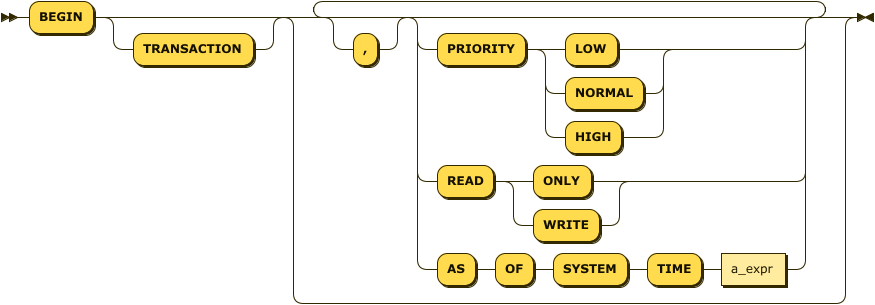
Figure 4-17. Begin Transaction
PRIORITY sets the transaction priority. In the event of a conflict, HIGH priority transactions are less likely to be retried.
READ ONLY specifies that the transaction is read-only and will not modify data.
AS OF SYSTEM TIME allows a READ ONLY transaction to view data from a snapshot of database history. We’ll come back to this in a few pages.
SAVEPOINT
SAVEPOINT creates a named rollback point that can be used as the target of a ROLLBACK statement. This allows a portion of a transaction to be discarded without discarding all of the transactions’ work. See ROLLBACK for more details.
COMMIT
The COMMIT statement commits the current transactions, making changes permanent.
Note that some transactions may require client-side intervention to handle retry scenarios. These patterns will be explored in Chapter 6.
ROLLBACK
ROLLBACK aborts the current transaction. Optionally, we can ROLLBACK to a savepoint, which rollbacks only the statements issued after the SAVEPOINT.
For instance, in the following example, the insert of the misspelled number ''tree is rollbacked and corrected without abandoning the transaction as a whole:
BEGIN;INSERTINTOnumbersVALUES(1,'one');INSERTINTOnumbersVALUES(2,'two');SAVEPOINTtwo;INSERTINTOnumbersVALUES(3,'tree');ROLLBACKTOSAVEPOINTtwo;INSERTINTOnumbersVALUES(3,'three');COMMIT;
The special savepoint cockroach_restart can be used to optimize transaction retries under certain circumstances. We’ll review this procedure in Chapter 6.
SELECT FOR UPDATE
The FOR UPDATE clause of a SELECT statement locks the rows returned by a query, ensuring that they cannot be modified by another transaction between the time they are read and when the transaction ends. This is typically used to implement the pessimistic locking pattern that we’ll discuss in Chapter 6.
A FOR UPDATE query should be executed within a transaction. Otherwise, the locks are released on completion of the SELECT statement.
A FOR UPDATE issued within a transaction will, by default, block other FOR UPDATE statements on the same rows or other transactions that seek to update those rows from completing until a COMMIT or ROLLBACK is issued. However, if a higher priority transaction attempts to update the rows or attempt to issue a FOR UPDATE, then the lower priority transaction will be aborted and will need to retry.
We’ll discuss the mechanics of transaction retries in Chapter 6.
Table 4-4 illustrates two FOR UPDATE statements executing concurrently. The first FOR UPDATE holds locks on the affected rows, preventing the second session from obtaining those locks until the first session completes its transaction.
| Session1 SQL | Session2 SQL | Comment |
|---|---|---|
BEGIN TRANSACTION |
BEGIN TRANSACTION |
|
SELECT * FROM numbers WHERE n=1 FOR UPDATE |
Data returned to Session1 and rows locked |
|
SELECT * FROM numbers WHERE n=1 FOR UPDATE |
Session2 waits |
|
COMMIT |
Data returned to Session2 and Session2 acquires locks |
|
COMMIT |
All locks released |
AS OF SYSTEM TIME
The AS OF SYSTEM TIME clause can be applied to SELECT and BEGIN TRANSACTION statements as well as in BACKUP and RESTORE operations. AS OF SYSTEM TIME specifies that a SELECT statement or all the statements in a READ ONLY transaction should execute on a snapshot of the database at that system time. These snapshots are made available by the Multi-Version Concurrency Control (MVCC) architecture described in Chapter 2.
The time can be specified as an offset, or an absolute timestamp, as in the following two examples:
SELECT*FROMridesrASOFSYSTEMTIME'-1d';SELECT*FROMridesrASOFSYSTEMTIME'2021-5-22 18:02:52.0+00:00'
The time specified cannot be older in seconds than the replication zone configuration parameter ttlseconds, which controls the maximum age of MVCC snapshots.
OTHER DATA DEFINITION LANGUAGE TARGETS
So far, we’ve looked at SQL to create, alter and manipulate data in tables and indexes. These objects represent the core of database functionality in CockroachDB as in other SQL databases. However, the CockroachDB Data Definition Language provides support for a large variety of other, less frequently utilized objects. A full reference for all these objects would take more space than we have available here – see https://www.cockroachlabs.com/docs/stable/sql-feature-support.html for a complete list of CockroachDB SQL.
Table 4-5 lists some of the other objects that can be manipulated in CREATE, ALTER and DROP statements.
| Object | Description |
|---|---|
Database |
A database is a namespace within a CockroachDB cluster containing schemas, tables, indexes and other objects. Databases are typically used to separate objects that have distinct application responsibilities or security policies. |
Schema |
A schema is a collection of tables and indexes that belong to the same relational model. In most databases, tables are created in the PUBLIC schema by default |
Sequence |
A sequence allows for the generation of unique numbers without requiring an explicit transaction. Sequences are often used to create primary key values, though, in CockroachDB, there are often better alternatives. See Chapter 5 for more guidance on primary key generation. |
Role |
A role is used to group database and schema privileges which can then be granted to users as a unit. See Chapter 12 for more details on CockroachDB security practices. |
Type |
In CockroachDB, a Type is an enumerated set of values that can be applied to a column in a CREATE or ALTER table statement. |
User |
A user is an account that can be used to log in to the database and can be assigned specific privileges. See Chapter 12 for more details on CockroachDB security practices. |
Statistics |
Statistics consist of information about the data within a specified table which the SQL optimizer uses to work out the best possible execution plan for a SQL statement. See Chapter 8 for more information on query tuning. |
ChangeFeed |
A change feed streams row-level changes for nominated tables to a client program. See Chapter 7 for more information on Changefeed implementation. |
Schedule |
A schedule controls the periodic execution of backups. See Chapter 11 for guidance on backup policies. |
ADMINISTRATIVE COMMANDS
CockroachDB supports commands to maintain authentication of users and their authorities to perform database operations. It also has a job scheduler that can be used to schedule backup and restore and timed Data definition changes. Other commands support the maintenance of the cluster topology.
These commands are generally tightly coupled with specific administrative operations, which we’ll discuss in subsequent chapters, so we’ll refrain from defining them in detail here. You can always see the full documentation for them at https://www.cockroachlabs.com/docs/stable/sql-feature-support.html.
| Command | Description |
|---|---|
CANCEL JOB |
Cancel long-running jobs such as backups, schema changes or statistics collections |
CANCEL QUERY |
Cancel a currently running query |
CANCEL SESSION |
Cancel and disconnect a currently connected session |
CONFIGURE ZONE |
CONFIGURE ZONE can be used to modify replication zones for tables, databases, ranges or partitions. See Chapter 10 for more information on Zone configuration. |
SET CLUSTER SETTING |
Change a cluster configuration parameter |
EXPLAIN |
Show an execution plan for a SQL statement. We’ll look at EXPLAIN in detail in Chapter 8. |
EXPORT |
Dump SQL output to CSV files |
SHOW/CANCEL/PAUSE JOBS |
Manage background jobs -imports, backups, schema changes, etc. - in the database |
SET LOCALITY |
Change the locality of a table in a multi-region database. See Chapter 10 for more information |
SET TRACING |
Enable tracing for a session. We’ll discuss this in Chapter 8. |
SHOW RANGES |
Show how a table, index or databases are segmented into ranges. See Chapter 2 for a discussion on how CockroachDB splits data into ranges. |
SPLIT AT |
Force a range split at the specified row in a table or index. |
BACKUP |
Create a consistent backup for a table or database. See Chapter 11 for guidance on backups and high availability. |
SHOW STATISTICS |
Show optimizer statistics for a table. |
SHOW TRACE FOR SESSION |
Show tracing information for a session as created by the SET TRACING command. |
SHOW TRANSACTIONS |
Show currently running transactions |
SHOW SESSION |
Show sessions on the local node or across the cluster. |
THE INFORMATION_SCHEMA
The INFORMATION_SCHEMA is a special schema in each database that contains metadata about the other objects in the database. You can use the information schema to discover the names and types of objects in the database. For instance, you can use the information_schema to list all the information schema objects:
SELECT*FROMinformation_schema."tables"WHEREtable_schema='information_schema';
Or you can use information schema to show the columns in a table:
SELECTcolumn_name,data_type,is_nullable,column_defaultFROMinformation_schema.COLUMNSWHERETABLE_NAME='customers';
The information_schema is particularly useful when writing applications against an unknown data model. For instance, GUI tools such as DBEaver use the information_schema to populate the database tree and display information about tables and indexes.
SUMMARY
In this chapter we’ve reviewed the basics of the SQL language for creating, querying and modifying data within the CockroachDB database.
A full definition of all syntax elements of CockroachDB SQL would take an entire book, so we’ve focused primarily on the core features of the SQL language with some emphasis on CockroachDB-specific features. For detailed syntax and for details of CockroachDB administrative commands, see the CockroachDB online documentation.
SQL is the language of CockroachDB, so of course, we’ll continue to elaborate on the CockroachDB SQL language as we delve deeper into the world of CockroachDB.
1 https://www.cockroachlabs.com/docs/stable/sql-feature-support.html
2 https://www.cockroachlabs.com/docs/stable/functions-and-operators.html
3 https://www.cockroachlabs.com/blog/using-lateral-joins-in-the-cockroachdb-20-1-alpha/
4 https://www.cockroachlabs.com/docs/stable/postgresql-compatibility.html
5 See https://www.cockroachlabs.com/docs/stable/online-schema-changes
6 https://www.cockroachlabs.com/docs/stable/bulk-delete-data.html