8
Causal Learning
In this chapter, we shall present an area of research in cognitive psychology which is attracting increasing attention, but which is rarely touched upon in the early years of university study, with a few exceptions in the context of animal learning (in which case the term “associative learning” is preferable to “causal learning” or, worse, “causal induction”).
We shall discuss what is currently meant by causal learning, starting with a brief history of the domain and a presentation of the key concepts.
The first research presented here (section 8.3) concerns adult subjects and relates to formalization efforts; section 8.4 deals with research on children. There are three main reasons for this order:
- 1) Research on children in this area concerns one of the very building blocks of thought: the construction of binary relations.
- 2) In adult subjects, with the exception of work focusing on modeling1, most publications relate to experimental situations featuring complex causal relations or situations defined in an arbitrary manner. For this reason, we have chosen to focus on the question of modeling causal learning mechanisms in our discussion of research on adults. Given the purpose of our book, it is important to be aware of this work on causal induction, which may be of interest to cognitive psychology students. Lay readers may wish to skip over this section or come back to it at a later date.
- 3) Section 8.4, which concerns research on children, also raises methodological questions about the domain of validity problem, and we shall outline our views on this subject here2. Some of our arguments will be presented in greater detail than others. The work presented in section 8.4 was chosen on the basis of three criteria: the experimental material used in all cases should belong to a similar family; it should be possible to present the experimental approach and arguments involved without going into too much technical detail; and the results of the research should provide interesting insights into the cognitive processes of causal learning.
8.1. Historical overview
In our opinion, the beginning of research into learning in cognitive psychology dates back to the mid-1950s, with work by Bruner et al. (1956). We have waited until this late stage in our book to present causal learning for historical reasons. Up until the last two decades, research into causal learning in human subjects was not particularly popular in the cognitive psychology community. More recently, interest has picked up again, with a rapid increase in experimental research and, at times, in heated debates. We shall not go into detail concerning these debates; in essence, they concern (a) identifying the theory and formalization that best account for the mechanisms and processes involved in causal learning3, and (b) the relations between causal learning and underlying processes found in other learning situations.
Living beings are reliant on the capacity to predict and monitor imminent states of their own environment in order to adapt and survive.
For example, a squid will project ink when it detects an approaching predator, but not for other marine animals. An observer might conclude that the squid has the capacity for causal attribution: but are they right to say this? In our view, the observer cannot be declared to be right or wrong until they have clearly defined what, for them, constitutes “causal attribution” behavior, and what does not.
To the best of our knowledge, experimental work in cognitive psychology began with the research of Piaget and Michotte.
Much of the published research in experimental psychology concerning causality in human subjects draws on the work of Michotte (1946). Although Michotte’s work is not always mentioned by name, almost all of the theoretical and experimental work presented in the current literature is based on an experimental paradigm that builds on Claude Bernard’s scientific approaches4. Michotte was essentially interested in physical and perceptive causality, and one of his very first publications in this domain still constitutes a point of reference5 for a large body of work inspired by the author’s research.
The term “causal attribution” is used here to refer to perceptive physical causality. A large amount of experimental research and theories in this area have focused on infants6, from newborn to around age 1. Most authors working in this field have concluded that even the youngest babies have the capacity for causal attribution: this lies at the root of the argument over nature/nurture (which is, in our view, not particularly helpful) or, to use more modern terminology, over the extent to which certain skills may be “hardwired”. In our view, “observables” collected from infants who have yet to acquire even the most basic linguistic comprehension skills suffer from excessive extrapolation. Almost all psychologists working in this field use the same few observation devices that are suitable for studying infants, but the axioms used in constructing measurement scales7 from the generated data have never been clearly defined. We may note that, as the number of publications using these devices increases, particularly with peer acceptance (especially if these “peers” have a certain academic reputation), the less likely it is that these devices will be called into question. In our view, this is an instance of the social consensus phenomenon that can occur in the humanities; we have therefore chosen not to present any research work based on observations of infants.
Piaget began to examine the question of causality in the mid-1920s. In his two main works on the subject (Piaget, 1927, 1971)8, the author examined the origins of causal attribution and causal reasoning, choosing to ignore the arguments relating to nature versus nurture and modularity9. Michotte, on the one hand, wished to determine the conditions of causal attribution10. Piaget, on the other hand, used the critical interrogation method with the aim of identifying the successive developmental stages involved in causal reasoning, along with the underlying mechanisms based on the constructivist theory, which he referred to as “genetic epistemology”. An explanation of these mechanisms lies outside of the scope of the information processing metaphor which forms the basis for this book.
8.2. Conceptual framework
We have chosen to adopt the general definition of a “causal relation” proposed by Michael E. Young (1995). A causal relation links two events (world states): an event c=cause and an event e=effect. The relation may be denoted by R(c, e).
According to Young (1995), the criteria used to define whether a relation is of the causal type are11:
- – temporal and spatial contiguity between c and e:
- a) event c must be immediately followed by event e,
- b) in terms of spatial and perceptive relations, two objects linked by a causal relation must be in contact, spatially, for a certain period of time;
- – temporal priority of c over e;
- – covariance, or rather contingency, of c and e;
- – prior experience.
8.2.1. Temporal and spatial contiguity
The question of temporal and spatial contiguity raises a further question in terms of defining the margin of variation in (1) the lapse of time between events c and e and (2) the distance between the two perceived objects c and e.
Should the time lapse between c and e be measured in milliseconds, or is a few seconds close enough?
In practice, the time lapse between two events c and e varies according to several factors. Two of these, which play an important role, are based on individual knowledge: (1) cases where the two events (objects) c and e are not familiar, and (2) cases where the causal relation is defined in an unfamiliar manner.
One example of the first case would be that of a person trying parasailing for the first time. They will observe that, once attached to the parachute, they will take off as the boat to which they are attached accelerates. The person may thus make a causal connection between taking off and the movement of the boat. However, if the individual in question is too caught up in enjoying the moment (or in fighting their fear), they will cease to focus on the way the boat is moving, and will not necessarily understand the reason for their more or less abrupt changes in altitude over the course of the experience, or for their safe landing back on the boat.
To illustrate the second case, consider Mrs. Smith, who is used to typing on a mechanical typewriter. She knows that in order to leave a space between two lines of text, she must turn the paper carriage roll upwards. Now, imagine Mrs. Smith starts using a word processing program on a computer. Much of her typing knowledge can be transferred directly to the new situation. However, in word processing, space is created automatically as the person types, and there is no need to insert fresh pages as the paper fills up. Mrs. Smith thus struggles to connect event “c”, a succession of inadvertent strokes on the spacebar or return key, with the event “e”, a white space of one or more lines between the last word she typed and the blinking cursor which indicates where the new text will be inserted.
In terms of spatial perceptive relations, spatial contiguity is generally an important cue in cases of movement transmission. According to Young (1995), following Leslie and Keeble (1987) and Schlottmann and Shanks (1992), very young children make inconsistent use of spatial contiguity cues, but this factor is important for causal attribution in adults and older children.
8.2.2. Temporal priority: cause before effect
If “temporal priority of c over e” is used as a criterion to decide whether causal attribution implies understanding of the causal relation, then it follows that subjects who are capable of causal attribution are also capable of establishing the correct order of c and e. Young (1995), citing Shultz, Altmann, and Asselin (1986) and Sophian and Huber (1984), among others, states that: (1) children under the age of 3 years do not consider this order as an important cue in understanding causal relations; (2) before the age of 3–4 years, “young children rel[y] on their prior experience rather than on temporal priority in deciding which of two objects was the cause and which the effect”. These results indicate a need for conceptual differentiation between causal attribution and causal inference behaviors. More recently, research conducted by Rottman et al. (2014) has shown that, in children under the age of 3 years, the direction of attribution between two objects X and Y (a cause and an effect) is inconsistent.
Finally, although temporal priority is, in theory, an important criterion in defining causal relations, there are cases where the temporal order of two world states does not indicate a causal relation between these states. For example, a baby may experience the succession of two temporally and spatially contiguous world states in unchanging order on multiple occasions, without there being a causal relation between these states:
EXAMPLE 1.– Mom puts the teat on the bottle full of milk; mom holds the bottle up to her cheek.
EXAMPLE 2.– A toy bear, a toy cat, then a toy rabbit emerge successively from behind a cushion placed in front of the baby. Each animal stays for three seconds, before being replaced by the next animal.
8.2.3. Contingency
Contingency may be defined as the conditional probability P(e/c), i.e. “the probability of e if c”. The difference between covariance and contingency is highlighted in the frequency Table 8.1.
Table 8.1. A case of contingency
| Presence of event E | Absence of event E | Total | |
| Presence of event C | 0.40 | 0.10 | 0.50 |
| Absence of event C | 0.10 | 0.40 | 0.50 |
| 0.50 | 0.50 |
Contingency: P(E/C) = P(C and E)/P(C) = 0.40/0.50 = 0.80
The majority of associationist theories encountered in the field of animal learning are based on a measure, ΔP (Jenkins and Ward 1965, cited by Holyoak and Cheng, 2011), known as the contingency model:
where:
P(e/c): the probability of e, given the presence of c;
P(e/-c): the probability of e, given the absence of c.
For the example given above, we have P(e/-c) = 0.20, so ΔPe = 0.60.
The value of ΔPe (= 0.60) may or may not be considered notable depending on the experimental hypothesis used in designing the observation procedure.
Other models have been proposed for human learning, such as Cheng’s power PC model (1997), which is a more specialized form of the contingency model, and, later, models based on Bayesian inference. The question of formalization in causal learning will be addressed in greater detail in section 8.3.1.
8.2.4. Prior experience
As we have seen, induction processes in human subjects are systematically based on a domain of knowledge that the individual already possesses. Prior experience determines a set of “expectations”12, limiting the number of causes to envisage and the memory load represented by the reasoning process13. Griffiths and Tenenbaum (2009) suggest that human subjects may use a “Monte Carlo” type heuristic, choosing to process a small sample of equally possible candidate causes each time; Holyoak and his colleague (see, for example, Lu et al., 2008; Powell et al., 2016) propose that we may be more likely to “bet” on a limited set of most likely causes.
Before a presentation of a selection of research on causal learning, it is important to clearly define three concepts that are often used, but rarely explained in detail, in these publications.
8.2.4.1. Causal attribution based on prior knowledge
This is the behavior that consists of expecting that a current event C will trigger an event E, and acting in consequence (e.g. seeing a large, unknown dog coming toward him, John quickly picks up the tiny kitten). This is also known as prognosis.
8.2.4.2. Causal inference or causal reasoning
This is the behavior that consists of selecting an unobserved event C from one’s knowledge base to explain an observed event E (e.g. on finding the garden wet one morning, Gertrude concludes that it must have rained during the night). This is also known as diagnosis. In certain cases, diagnosis allows us to act on causes in the most economical manner. For example, we know that a battery-operated device ceases to operate when the batteries are empty, although the failure may have other causes. Faced with a device that ceases to operate, people check the batteries before considering any other possible causes of device failure.
8.2.4.3. Causal induction or causal learning
Causal induction or causal learning, the main theme of this chapter, consists of creating a structure of relations between a set of observations that are interconnected by certain criteria. The concept of induction is also used to denote the cognitive process that produces knowledge which the individual may then incorporate into their knowledge base (i.e. long-term memory) for the purposes of causal attribution (defined in 8.2.4.1).
8.3. Formalization and experimental research on adults
Causal reasoning is one of the most vital cognitive abilities, used in everyday life in our physical and social environment. It forms the basis for enriching our pragmatic and scientific knowledge. As we have seen, causal learning has only been considered as a field of research in its own right within the sphere of cognitive psychology for around 20 years. We will not present all of the different approaches to theorization and formalization presented in the literature here: interested readers may wish to consult publications by Waldmann and Hagmayer (2013) and Sloman and Lagnado (2015), which require some prior knowledge of cognitive psychology (master’s level).
In this section, we shall give a conceptual presentation of the Bayesian model, which currently dominates the discussion of causal learning. We begin with a brief outline of the history of this model, which belongs to the probabilistic class and has its roots in the behaviorist approach to animal conditioning. We shall then present two recent research projects based on the Bayesian model of causal induction, conducted by Bonawitz et al. (2014) and Powells et al. (2016).
8.3.1. Probabilistic models of causal learning
Causal learning models have their origins in the associative models used to study conditioning in animals.
The idea of using animal conditioning models to study causal learning stems from the fact that, in conditioning, an animal will react spontaneously to a certain number of unconditioned stimuli (a stimulus is an event that occurs at a given moment: for example, if a hungry dog kept in a cage sees a piece of meat, it will salivate; this response is “unconditioned”, as it is spontaneous).
Conditioning consists of introducing a conditioned stimulus, such as the sound of a bell ringing, in advance of the unconditioned stimulus. Following a certain number of iterations, the dog will start salivating when it hears the bell. In neutral terms, the animal is said to be conditioned to the unconditioned stimulus (the sound of the bell). Based on this observation, the experimenter concludes that the animal has “learned” to salivate when the bell rings. This is an interpretation of an observed behavior, giving the behavior the status of a psychological phenomenon.
8.3.1.1. Associative models
Associative models were used before the emergence of the symbolic information processing approach in cognitive psychology. We touched on this theme briefly earlier. It is interesting to note the series of books entitled Handbook of Learning and Cognitive Processes, edited by William Estes, a major player in the field of learning14. In the five titles published between 1975 and 1978, all the formalized models of learning included were probabilistic models, despite the increasing popularity of the information processing approach at that time.
Probabilistic models became increasingly rare in human learning studies from the 1970s onwards, but remained popular in the field of animal learning, with one notable example being the Rescorla–Wagner model (1972). This model was taken up and adapted for human learning from the mid-1980s onwards. The first research using probabilistic models for humans focused on contingency judgment (e.g. Schanks, 1985). The ΔP model for human learning, mentioned in the introduction, was adapted by Patricia Cheng (1997)15, who added two assumptions concerning the nature of the causal relation: (1) causes are independent; (2) their causal power may be expressed by a probability that evolves in relation to their margin of variation.
All of these models simply ignore one aspect of causal induction in humans: prior knowledge. This fundamental notion was finally introduced as part of the Bayesian model.
8.3.1.2. The Bayesian model of human learning
The determination of a causal relation is based on the concept of covariance of the cause and the effect. Causal induction thus implies estimation of the strength of a relation.
The research on human subjects presented in section 8.4 shows that we require very few observations to induce causal relations (correct or otherwise). This makes it critical to presuppose the existence of prior knowledge before any observations of situations that incite individuals to infer a causal relation. The variation in the minimum number of observations needed to induce a causal relation depends on this prior knowledge. Furthermore, it is important to distinguish between causal structure and the strength of a causal relation. Human subjects have a strong tendency to look for a cause when confronted with a more or less new observation, i.e. to infer a causal structure. This causal structure is drawn spontaneously from prior knowledge.
Building on the idea that prior knowledge is fundamental in causal inference, the Bayesian model presupposes that subjects will adopt a set of hypotheses concerning causal structures according to an a priori distribution of probabilities in contexts of causal learning.
Unlike artificial systems, human subjects have a limited working memory capacity. We cannot therefore presume that individuals are able to manage large sets of hypotheses. From the outset, a subject will adopt a small set of hypotheses from those which they consider most likely. These hypotheses are examined in light of the observations, and re-evaluated using the “update” process in the Bayesian model16.
The result of this update is a new, a posteriori distribution, produced by choosing a new limited set of hypotheses.
The crucial question to address here concerns the criteria used in choosing a new set. From the 1960s onwards, authors creating models based on the associative approach predicated the existence of a choice strategy for new hypothesis sets based on two criteria: coherency with observations, and likelihood.
In cases where observations do not contradict hypotheses based on prior knowledge, no change is made. Bruner et al. (1956), in the work presented earlier, showed – without reference to probability – the existence of two strategies in simple concept-identification tasks in a laboratory setting: focusing and scanning. Focusing strategies are most common in adults, while scanning is more frequently observed in children. In a later article (1975), Bruner et al. demonstrated that adults make use of both strategies in the context of more complex problems. Using a scanning strategy, subjects retain a hypothesis as long as it has not been contradicted by an example, choosing an alternative option only when they observe a negative example.
The majority of recent publications involving formalization draw on the Bayesian model, with a few variations. One of these variations concerns the possibility of forgetting one of the pre-selected hypotheses that has proved incoherent with observations in the past: in other words, faulty subject memory. Without going into detail, we shall see, in the first research case presented below17, that the choice of a model to use in experimental research may lead to the adoption of a questionable data elaboration method (but which adheres to that model). In this case, the model in question is a Bayesian variant in which subjects are presumed to have an excellent memory of observables, leading to faultless updating of hypothesis sets.
Given our aim of presenting research in a way that limits the need for technical knowledge, this time in the field of probability calculations, we should simply note one fundamental difference between classical associative models and the Bayesian model: in the latter case, the probability of different hypotheses before observation (a priori probability) is not equal. The probability distribution is revised following one or more observations according to the degree of coherency between hypotheses and observables (a posteriori probability). The model enables us to calculate these a posteriori probabilities, i.e. the likelihood of a given hypothesis, denoted by P(h/d)18. In human learning, unlike machine learning, we assume that subjects will work with a small set of hypotheses. Researchers using this model may choose to base their observations on one of two strategies: the choice of a new set of hypotheses from prior knowledge following each observation or a series of observations, or an update procedure that takes account of previously observed data. In the second case, researchers choose whether or not to presume that the subject has a good memory for prior experiences.
8.3.2. Two examples of research on adults
8.3.2.1. Strategies used to select cause hypotheses: Bonawitz et al. (2014)
The authors of this research presented a Bayesian model with two predicates: (1) subjects adopt a scanning-type strategy, as proposed by Bruner et al., i.e. retain a hypothesis as long as it has not been contradicted by observations. This strategy is known as WSLS (Win-Stay, Lose-Sample); (2) subjects successfully memorize observed data, which is then used to update a priori hypotheses.
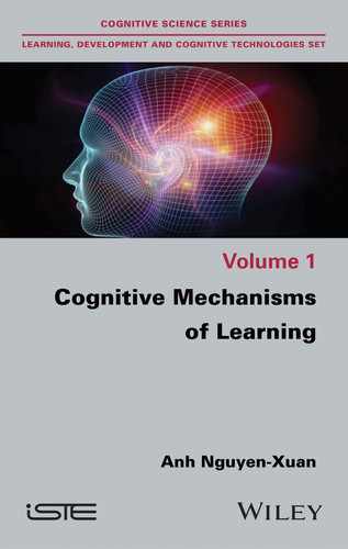
To illustrate their model, the authors carried out research on adult students and children aged 4–6 years. The experiments involved blicket detector-type artificial laboratory situations19. The prior knowledge involved20 did not stem from the subject’s real-world experience; it was detected as part of the experiment itself, as we shall see in the first part of the experiment, common to the two experimental procedures P1 and P2 (for a “measure” of artificial prior beliefs).
The published article, intended for a specialist audience21, the description of the material used and the presentation of data feature a number of omissions. In this section, we have chosen to present two experiments: the first (experiment 1) concerned a group of 30 adults, and is reported in greater detail than experiment 2. The presentation of this second experiment would need to be rewritten in considerably greater detail to render it accessible to non-specialist readers; we shall simply provide a brief summary here.
Experiment 1 was designed to test the model in a determinist situation. The authors stated that this determinist situation is simply an approximation of real situations, and was chosen to assess the feasibility of the selected type of experimental approach.
In experiment 1, the causal relation was therefore presumed to be determinist, with the likelihood value of a hypothesis h set at either 1 or 0: P(d/h) = 1 if an observation d is consistent with the hypothesis h, otherwise P(d/h) = 0.
The 30 adult participants were split into two groups, Ga and Gb. Ga completed the experiment following procedure P1, then following procedure P2; Gb completed the experiment in reverse order. The experiment comprised two phases: (1) an evaluation of prior beliefs and (2) the observation of an event and the choice of hypotheses concerning its causes.
8.3.2.1.1. Evaluation of prior beliefs
The responses given by subjects during this phase were used to group them into categories according to their beliefs regarding the causes of an event.
The experimenter showed the subject six blocks. Three were painted red on all but one face, while the other three were painted yellow on all but one face. Each block had a hidden switch on the back which the experimenter (E.) could flip to surreptitiously light up the block.
E. told the subject that when a red and a yellow block are bumped together, either both will light up, one will light up, or neither will light up. However, if two blocks of the same color are bumped together, either both will light up or neither will light up. The subject was asked to help E. to discover how the blocks work.
E. then asked the subject three questions22:
- a) “If two red blocks are bumped together, will they both light or both not light?” Subjects responded by pointing to the chosen response drawn on a card (both light/both do not light). The non-chosen card was removed, and the chosen card left on the table.
- b) The same question, but for two yellow blocks, with the same response choice procedure.
- c) The same question, but for one red and one yellow block. This time, there were four possible answers (red lights, yellow lights, both light, both do not light).
Subjects’ answers to these questions (before any observation events) were taken as measures of their beliefs (prior knowledge) concerning the block activation rules.
8.3.2.1.2. Hypothesis choice behaviors
E. showed the subject a single event. Group Ga completed procedures P1 and P2 in that order, while group Gb completed the procedures in reverse order.
Procedure P1: E. took a red block and a yellow block and bumped them together. Only the yellow block lit up.
Following this single event, E. asked the subject two questions, noting their responses:
- 1) What will happen if I bump two red blocks together?
- 2) What will happen if I bump two yellow blocks together?
Procedure P2: E. took a red block and a yellow block and bumped them together. Both blocks lit up.
Following this single event, E. asked the subject two questions, noting their responses:
- 1) What will happen if I bump two red blocks together?
- 2) What will happen if I bump two yellow blocks together?
The experimental process is shown in Figure 8.1.
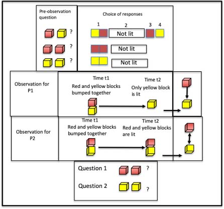
Figure 8.1. Illustration of experiment 1. For a color version of this figure, see http://www.iste.co.uk/nguyen/cognitive.zip
The most important prediction specific to this model is as follows. Given an initial hypothesis favoring one of the 16 possible causal structures23: 1) if the observation is compatible with the previously selected structure, then this structure will be retained, and the answers to the two questions following the observation will be the same as those given previously; 2) if the observation is not compatible with the previously selected structure, then the subject will not choose an alternative at random from the set of 16 possibilities, but will choose one that is compatible with their observation (P1: only the yellow block lights; P2: both the red and the yellow block light).
Subjects’ responses to questions (1) and (2) are classed as either compatible or incompatible with one of the four causal structures potentially corresponding to the observation.
The hypothesis space and hypothesis structures that are compatible with responses given in procedures P1 and P2 are shown in Figure 8.2. This figure is a reconstruction based on the laconic description of the classification method provided by the authors.
For both P1 and P2 procedures, the structures that answer to questions (1) and (2) can be classified as belonging to the compatible structures are respectively: for (P1) 2, 6, 10, 14; and for (P2) 4, 8, 12, 16.

Figure 8.2. The 16 possible causal structures. For a color version of this figure, see http://www.iste.co.uk/nguyen/cognitive.zip
The authors did not include a table in their article to provide the number of compatible or incompatible answers. Instead, they provided a graphic showing the path taken by each individual from the first structure they chose to the structure chosen in response to post-observation questions (1) and (2). Upon examination, we see that only 1 out of 60 subjects gave a response that did not correspond to one of these four structures. The authors considered that these results were conclusive regarding the feasibility of later experiments based on their probabilistic model, which is better suited to studies of causal induction in real life. Experiment 1 was simply an approximation of real situations.
Recall that experiment 1 was designed to test the model in a deterministic situation, considered as an approximation of real situations, but one which was necessary to test the feasibility of this type of experimental approach. It would thus be reasonable to expect collected data to conform less precisely to the predictions made by the model.
It thus seems reasonable to wonder why the results correspond to the predictions made by the model to such an impressive extent.
We thus took a closer look at the way in which responses to questions (1) and (2) were classified. Note that the only observation made before these questions concerned contact between one red block and one yellow block. The two questions concerned what would happen in case of contact between two red blocks and in case of contact between two yellow blocks. Figure 8.2 shows the way in which responses were classified as “compatible” or “incompatible”.
The compatible hypothesis structures for procedure P1 are 2, 6, 10 and 14, as shown in Figure 8.3.
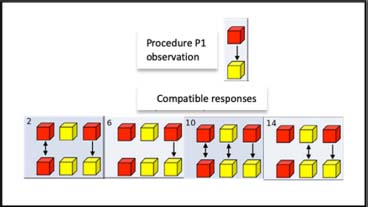
Figure 8.3. The four compatible structures. For a color version of this figure, see http://www.iste.co.uk/nguyen/cognitive.zip
From Figure 8.3, we see that the responses “both red blocks light” and “both yellow blocks do not light” are considered to belong to compatible structure 2; the responses “both red blocks do not light” and “both yellow blocks do not light” are considered to belong to compatible structure 6, etc.
However, we wonder which “incompatible” structures also include response pairs found in structure 2 (or 6, 10 or 14). Figure 8.4 shows the case of structure 2.
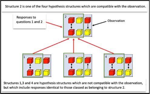
Figure 8.4. Incompatible structures 1, 3 and 4. For a color version of this figure, see http://www.iste.co.uk/nguyen/cognitive.zip
Procedure P1
- – Structure 2: responses “both red blocks light, both yellow blocks do not light”. The same responses are found in structures 1, 3 and 4.
- – Structure 6: responses “both red blocks do not light, both yellow blocks do not light”. The same responses are found in structures 5, 7 and 8.
- – Structure 10: responses “both red blocks light, both yellow blocks light”. The same responses are found in structures 9, 11 and 12.
- – Structure 14: responses “both red blocks do not light, both yellow blocks light”. The same responses are found in structure 13.
We see that without taking account of the previous observation (red does not light, yellow lights), the responses to questions (1) and (2) may correspond to any of the 16 hypothetical structures.
Procedure P2
- – Structure 4: responses “both red blocks light, both yellow blocks do not light”. The same responses are found in structures 1, 2 and 3.
- – Structure 8: responses “both red blocks do not light, both yellow blocks do not light”. The same responses are found in structures 5, 6 and 7.
- – Structure 12: responses “both red blocks light, both yellow blocks light”. The same responses are found in structures 9, 10 and 11.
- – Structure 16: responses “both red blocks do not light, both yellow blocks light”. The same responses are found in structures 13, 14 and 15.
Once again, we see that without taking account of the previous observation (red lights, yellow lights), the responses to questions (1) and (2) may correspond to any of the 16 hypothetical structures.
Bonawitz et al. did not query their choice of method for classifying individual responses, and failed to ask why their results corresponded almost perfectly to the predictions made by their model. They stated that the experimental results24 that they obtained did not provide a solid foundation to test a probabilistic model25. However, they considered that their experimental approach provided a suitable basis for developing experimental situations with the capacity to handle stochastic cause/effect observations.
In experiment 2, the same type of material was used in a blicket detector situation26. The experimenter placed red, blue or green blocks in a blicket detector next to a light-up helicopter toy, which switched on or remained off in different cases.
During the assessment phase for prior beliefs, an initial probability for each type of block was suggested by showing subjects 18 different cases in which a block of a given color (red, blue or green) was placed in the detector. The red block resulted in the helicopter lighting up five times out of six. The green block had this effect three out of six times, and the blue block only resulted in the helicopter lighting up on one of the six occasions. The experimenter then showed the subject a white block, stating that it was a colored block that had lost its color. The subject was asked to guess the original color of the block. Next, the block was placed into the detector, which lit up or did not light up (according to one of the two experimental conditions, with 60 students split into two groups). The procedure was repeated four times using four white blocks.
The observed data from this second experiment (i.e. subjects’ successive choices concerning the original color of each white block) consisted of aggregations of individual choices over the four observations. This data was compared to the behaviors displayed by the Bayesian model in two opposite cases: the model either chose a hypothesis at random on each occasion (the IS, Independent Sampling, strategy), or adopted the WSLS (Win-Stay, Lose-Sample) strategy. The correlation between the experimental results (aggregations of individual data for the four tests) and the predictions made by the model using the WSLS strategy was higher than for predictions using the IS strategy.
Note that, as in the case of all highly specific research on causal induction in adults, this work would be improved by including a more explicit presentation of the data elaboration methods used.
Because of the rather imprecise way in which the data elaboration method used in the first experiment was presented, we took a closer look at this methodology. We attempted to understand, on the one hand, why the authors declared that probabilistic methods are better suited to explaining causal induction in humans, and on the other hand why they did not seek to find out why the data collected using a determinist causal induction situation corresponded so closely to the predictions made using a probabilistic model.
We can only wonder why the peer reviewers of this article – published in one of the most prestigious cognitive psychology journals – did not ask the same questions.
8.3.2.2. The main cognitive bias in causal learning: Powell et al. (2016)
Staying with the Bayesian model, Powell et al. (2016) studied the effect of a highly general cognitive bias, frequently observed in causal inference situations featuring more complex laboratory cases, and which draw on the prior knowledge of a given subject population. These laboratory situations are considered to provide a closer approximation of real life.
In this article, the authors proposed that a cognitive bias known as “sparse and strong priors” should be taken into account in the context of causal learning by human subjects in real-world situations. This bias is a cognitive efficiency principle: if subjects find themselves in a situation where they must attempt to explain why an observed event took place, they will tend to consider a reduced set of strong, familiar causes (and, unless otherwise noted, the first cause to emerge is often determinist in nature). The Bayesian model put forward by the authors predicts that, given a set of independent and competing causes, subjects will tend to exaggerate the strength of the cause with the highest observed frequency and to underestimate the strength of the least frequently observed cause.
In this section, we shall present two experiments conducted by Powell et al. on causal learning in a complex situation with several possible non-determinist causes:
- 1) A case with two competing possible causes, A and B: this is somewhat closer to real-life situations in which a situation X (this egg is not fit for consumption) may be the result of several independent causes (it was cracked when it was collected three days ago/the chicken which laid the egg is sick).
- 2) A case involving the induction of “preventive causes”: in real life, both desirable and undesirable effects have causes. If an undesirable effect is canceled out by the presence of another cause, then this cause is said to be “preventive”.
8.3.2.2.1. Induction of competing causes
This experiment27 concerns the induction of a given cause A in the presence of a competing cause B. The authors compared subjects’ estimations of the strength of these cases: (a) when competing cause B is highly likely or highly unlikely; (b) when subjects were presented with a small number of observations, or with a higher number of observations (double or triple the original quantity).
In complex induction situations featuring several potential causes, the number of observations required is highly variable depending on the number of causes, the respective probabilities assigned to each of these causes and the number of types of combinations of causes that are available. Without going into technical detail, the procedure may be described in the following manner. Contingency tables are used for the probability values assigned to each cause, and for the degree of dependency between these causes. Given N possible causes, the number of possible combinations is the power set of N (i.e. the set whose members are all of the possible subsets of N). With three or more causes, the number of possible combinations begins to increase dramatically (16, in the case where N = 3). To reduce the number of observations the subject must have observed in order to perform their inductive reasoning, the authors selected combinations that define a minimum number of observations, respecting the cause existence criteria and the probability of these causes. This minimum number may then be doubled or tripled as required for the experiment in question.
In this case, as in most experimental research on causal induction, subjects were presented with sequences of situations28, including one or more possible causes and an effect which is either present or absent.
The experiment was carried out with 114 undergraduate students who were split into two groups (G1 and G2). The experimenter told each subject that their task was to help a doctor to define the cause(s) of an illness, based on a series of files for individual diners at a restaurant, all of whom ate a certain dish, some of whom fell ill. The cover story was as follows:
“Many of the guests at [a] new resort have become ill […]. Every day, at dinner, the resort provides a complimentary salad for its guests. The salads can be made with different exotic vegetables. The resort’s doctor thinks one or perhaps several of these exotic vegetables [pictures shown: vegetables A, B and C] may be causing the illness. You will be reviewing a number of case files that describe what a guest ate and whether they became sick…”
The case files took the following form:
[Mr. X ate a salad including plant C (or plants A and C; plants B and C; plants A, B and C); Mr. X is sick (or is not sick)].
E. showed the subject a series of files (a block of 44 individual files), followed by a picture of a plant. They then asked the subject the following question: “Imagine 100 healthy people ate this vegetable. How many do you estimate would get sick?” The question was repeated for each of the vegetables.
Three blocks of 44 files, concerning a total of 132 clients, were constructed. Each block contained the same proportion of files with each vegetable combination29.
The main criterion used in developing the file set was that causes A and B were in competition, and that they were independent.
Four combinations of potential causes (four types of salad) were used: [with C], [with A and C], [with B and C] and [with A, B and C]. Additionally, a contingency table was constructed in which causes A and B were independent. The proportion of different types of individual files (out of a total of 44 files per block) was based on the following probabilities for the three causes:
- 1) For group G1 (57 participants): probability of C=0.09 (very weak); probability of A=0.50; probability of B=0.80 (strong probability).
- 2) For group G2 (57 participants), the probabilities of C and A were the same as above; however, the probability of B = 0.20 (weak probability).
Examples of file types:
[Mrs. Anderson: ate plant C, is sick] (1 file).
[Mr. Andrews: ate plant C, is not sick] (10 files).
[Mr. Bernard: ate plants A and C, is sick] (6 files).
[Mr. Daniels: ate plants A and C, is not sick] (5 files).
The data from groups G1 and G2 was compared to assess their estimation of the strength of each cause (with a strong or weak cause B).
For the first block, group G1 (weak B) estimated the strength of cause A to be greater than 0.5; group G2 (strong B) estimated the strength of A at under 0.5. The difference between these frequencies was significant. Given two possible causes A and B, the strength of a cause (A) was estimated to be high if the competing cause (B) had a weak probability. However, the estimated strength of A was lower when the competing cause B was much more probable. This difference between groups G1 and G2 ceased to be significant once subjects had seen two blocks (88 files in total) and remained insignificant after three blocks (all 132 files): estimations of the strength of A from both groups converged toward a value of p=0.50. This result in terms of cause A corresponds closely to the predictions made by the model.
The experimenter asked subjects to estimate the strength of cause C, something which they might not have done spontaneously. The probability of C was very weak (p= 0.09); participants systematically overestimated the strength of this cause. This overestimation did not vary over the three blocks (with a mean strength oscillating between 0.2 and 0.3, with very low inter-individual variation). This tendency is also compatible with the sparse and strong priors bias.
In the case of a weak B (p = 0.20), participants overestimated the strength of this cause over all the three blocks (with a mean oscillating between 0.35 and 0.4). However, the strong B group (p = 0.80) significantly underestimated the strength of B throughout the three blocks. The authors did not examine this last finding in any detail.
We propose two types of interpretation. The first relates to the common regression toward the mean phenomenon, but this statistical effect is not linked to any psychological process. The second type of interpretation is psychological in nature, but predicated on the (debatable) idea that all individuals in the group process information in the same way. The subjects involved in this experiment were adult students who were asked to estimate the strength of three possible causes on a scale from 0 to 100. It is entirely possible that they believed the numbers to correspond to proportions out of 100, meaning that the total of the three strengths could not exceed 100. In this case, the strength of A (with an a priori probability of 0.50) was estimated “correctly”30; if the strength of C was estimated at an average value ranging between 0.20 and 0.30, we would then expect the estimation for B to be coherent with a total of 1.00, i.e. well below 0.80.
8.3.2.2.2. Induction of independent and competing preventive causes (experiment 3)
In this experiment, the authors aimed to examine what would happen with two types of co-existing causes: causes triggering a given situation, and causes preventing this situation from occurring when present. The causal induction situation is complex, as it included one cause which may result in sickness, and two competing but independent preventive causes. Furthermore, in this experiment, subjects were not informed of the direction of each cause, i.e. which of the three plants were toxic and which had a preventive effect.
The material used in this case was similar to that for the previous experiment. There were four salad options: [C], [A and C], [B and C] and [A, B and C]. Subjects were told: “One or more of the vegetables could be making the guests sick. However, not all of the guests who ate salad are getting sick. One or more of the vegetables may have medicinal properties that prevent the illness”.
E. presented subjects with a series of files, then with representations of plants A, B and C. Each time, subjects were asked how many guests, from a total of 100, they would expect to fall ill after eating the plant. If (and only if) subjects indicated that a given plant had a preventive effect, E. asked them to estimate the strength of this effect on a scale from 0 to 100: “Suppose 100 people are about to get sick. If they all eat this vegetable, how many of the 100 will not get sick?” If a participant simply indicated that the vegetable in question was not a cause (preventive or otherwise), then a strength rating of 0 was assigned.
Files were constructed using contingency tables, taking vegetable C to be a cause of sickness and vegetables A and B to have preventive effects, although independently of one another (both are preventive, but their effect was not cumulative). Students were split into two groups of 57: G1 and G2. The probability of cause C was high, with p = 0.80, and the probability of cause A was 0.50. For cause B, two probabilities were used: a weak probability of 0.25 (group G1) and a strong probability of 0.75 (group G2). Three blocks of 40 files were used, with equal proportions and distributions of files, as before.
Overall, and in contrast to the previous experiment, the competing preventive cause B was seen to have an effect on the estimation of the strength of preventive cause A over all the three blocks. The strength of A was always underestimated by the strong B group. This result is not coherent with the predictions made by the model. The authors noted a major difference between experiment 3 and their previous two experiments, in that participants had no prior knowledge of the polarity of causes (generative/preventive). In the case where B was a weak preventive cause (0.25), certain subjects may have mistaken the polarity of this cause, or considered B to have no effect on the observed events. These results were taken into account in the model which the authors presented later in their article (which will not be described here).
In our view, the concept of a preventive cause itself may have played a role in experiment 3. The problem-solving situation used in experiment 3 is more complex than that used in the two previous experiments, as subjects were required to think about causes which may act in different ways. Vegetable C causes sickness with a probability p. If this is the only vegetable in the salad, then people who eat the salad will get sick with a probability p. If the salad includes both C and A, there is a weaker probability of the guest becoming ill. The complexity lies in understanding what we mean by the term “preventive cause”, as this may refer to several possible cases.
Let us say that C is a “toxin” and A an “antidote”. Antidotes may operate in several different ways, principally: (1) by neutralizing the effect of the toxin: A changes the nature of C, with which it forms a non-toxic compound, reducing the total quantity of ingested toxin. For example, an acid derived from sulfur combines with mercury to form an inert molecule which the organism is able to eliminate (chelation); (2) by correcting the effects of the toxin. For example, there are several possible causes of hypoglycemia, including the ingestion of certain quinine derivatives. The effects of hypoglycemia are corrected by the consumption of glucose.
It is thus entirely possible that different subjects did not understand the concept of an “antidote”, i.e. a preventive cause, in the same way.
8.3.3. Causal learning in adults: conclusion
Once again, we wish to make the following point regarding the “validation” of a model by comparing it to observed data. In these cases, statistical tests are almost systematically used, and with group data31. This comment is particularly relevant in the case of models based on probability calculations, which can only be tested by aggregating observations of individual behaviors. Researchers may conclude, based on results obtained from group observations and a statistical model, that results are or are not acceptable, with a probability p (confidence threshold). However, a group is not an individual; group values represent an “average” individual according to one or more measurement scales.
Given the generalization of the Bayesian model for studying causal learning, it is interesting to note the following reflection32 by Sloman and Lagnado (2015), who propose the creation of a general journal of causal thought. According to the authors, the Bayesian model of causal induction (CBN, Causal Bayesian Network) both over-and underestimates human reasoning capacities. On the one hand, humans have a limited working memory capacity, notably in terms of estimating the probability distribution of a set of hypotheses. On the other hand, the CBN model does not explicitly take account of a variety of spatio-temporal information elements, of similarity, etc. Sloman and Lagnado (2015) do not question the relevance of the CBN model: instead, they consider it as a starting point for formulating a better psychological theory – but not as an end in itself.
To conclude, we would point out the following general results from the research work in causal learning in adults. In principle, for any given individual, causal induction involves the aggregation of a series of observations, which may be spaced out over time. It is thus difficult to recall all of the different structures and causal relations that may be at play, and may compete, in our reasoning. Human subjects thus tend to make simplified assumptions, and to suggest a single cause for any observed event.
In terms of causal attribution, individuals tend to look for familiar causal structures within their store of prior knowledge. The richer a person’s prior knowledge (e.g. if we compare an adult to a child), the more likely they will be to draw on this knowledge; in certain cases, prior knowledge may prevent us from inducing causal structures and/or relations in unexpected or artificial situations. This has been observed in laboratory situations, where adults emit hypotheses about causal structures that are not those intended by the researcher (see, for example, Lucas et al. 2014).
Furthermore, we tend to prefer causes that cover the greatest number of effects. In cases with several competing causes, we use an elimination strategy, seeking evidence to use in eliminating certain options. For example, leaving the house in the morning, if I find the sidewalk wet, my first thought is that it has rained recently; I expect that the sidewalk in the next street, where my car is parked, will also be wet, and that there will be raindrops on my car windshield. However, if I turn the corner to find a dry street, the “recent rain” cause is no longer probable, and I switch to another option: “the street cleaner has just passed through”.
In terms of the adoption of a causal structure connecting two situations in terms of “cause situation” and “effect situation”, we tend to adopt simple structures, i.e. binary type relations. Furthermore, in cases with multiple causes, we prefer to assume that these are independent; conjunctive structures (where several simultaneous causes are required to produce an effect) are rarely mentioned, except in very unusual cases.
8.4. Experimental research on children
In order to assign “cause” and “effect” roles to two events, we must first understand that these two events are linked by a relation. In the 1970s and 1980s, following on from Piaget’s work on the construction of logical thought around seriation and classification during the concrete operation stage, we carried out a series of experimental research projects on problem-solving and learning to solve problems related to asymmetric transitive binary relations (e.g. “Andrew is taller than Bernard”) in seriation33 and symmetric transitive binary relations (e.g. “Andrew is with Bernard”) in classification34.
Recall that in Piaget’s theory of cognitive development, logico-mathematical thought is constructed progressively over the course of three stages, linked to three hierarchical levels: the preoperational stage, the concrete operational stage and the formal operational stage. The two logical grouping processes, seriation and classification, are established during the concrete operational stage. Acquisition of number stems from the coordination of these two processes, which Piaget described in terms of logical structures.
However, a logical structure is simply a representation of fundamental mechanisms and is not sufficient to describe operating processes in specific problem-solving situations that require subjects to handle objects linked by binary relations. The work mentioned above, conducted from an information processing perspective, was intended as a complement to the Piagetian approach. We examined the operating process dimension of these processes, which varies according to the problem situation. For example, the processes involved in constructing a series of three terms (Nguyen-Xuan, Rousseau and Lemaire, 1974) are different from those involved in constructing a series of more than three terms (Nguyen-Xuan and Rousseau, 1976)35. We also highlighted the astonishing flexibility of human intelligence, which essentially aims to reduce mental load at all times36. Participants were notably seen to change the solution strategy between two problems that were structurally isomorphic37, but subject to different constraints relating to the way in which objects could be handled (Nguyen-Xuan and Hoc, 1987) or in the way of obtaining information concerning these binary relations (Shao and Nguyen-Xuan, 1994).
The binary relations that we studied are generally established at around 7–8 years of age, in problem situations that involve verbal instructions and require relatively complex coordination between information, delivered sequentially, and the actions that a subject may carry out on one or more objects. More recently, other authors have examined the way in which more “primitive” binary relations, such as “above/below” or “same/different”, are acquired.
In this section, we shall provide a more detailed presentation of research carried out on young children. The main reason for this is that a causal relation may be very simple or very complex: from a simple [single cause/single effect] relation to a [causal chain with multiple conjoined/disjoined causes] relation.
The question of domains of validity in cognitive psychology (as in many other social sciences) is particularly relevant in research on children which is designed to identify the age at which specific knowledge is acquired. In choosing research to present here, our aim was to illustrate the current state of experimental work in this area with the least possible technical detail. We shall also use this work as a starting point for discussion on the “domain of validity” question, which we consider to be fundamental in the context of experimental cognitive psychology.
Some experimental work on key questions concerning the development of causal thought is presented below.
8.4.1. The above/below relation
Christie and Gantner (2010) studied problem situations directly related to learning a primitive binary relation: above/below (specifically, in this article, “white thing above black thing, otherwise identical”). This situation is similar to that used in a concept-identification experiment38 in which the experimenter showed two positive examples of a concept, then asked a subject choose between two other options, one belonging to the concept, the other not belonging to the concept. The aim of this experiment was to show that children are capable of learning the relation from age 3, but only if the positive examples are presented at the same time. A brief presentation of some of the material used and some of the experiments carried out, responding to the authors’ initial questions, is given below39.
The experimental material consisted of eight sets of images. Each set included one pair of “standard” (learning) images, both positive examples, and a pair of “alternatives” (test images), one of which was a positive example, the other being an example that did not belong to the concept. Each pair of standard images (positive examples) featured two identical, familiar animals (e.g. two dogs), one above the other. The only difference between the two animals was their color: one was drawn in black on a white background, while the other was drawn in white on a black background. For the alternative images, the first (a) was a positive example (“relational match”), featuring two images of a new familiar animal (such as a bird), identical in all but color, placed one above the other. The second alternative image (b) showed an example that did not correspond to the concept, featuring two animals of the same color, one of which featured in the first standard image, the other being featured in the second sample image. These animals were placed diagonally from one another. A copy of a figure from the article (1975) is shown in Figure 8.5.
The aim of this research was to compare two experimental conditions: the sequential situation and the comparison situation.
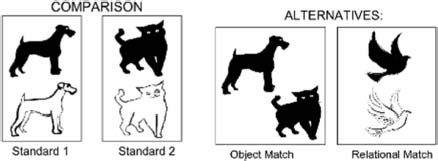
Figure 8.5. One of the eight image sets corresponding to one of the eight verbal labels
In the sequential situation, the two standard images were presented one after the other. When presenting the first standard image, the experimenter (E.) used an invented word, or “label”, to denote the image: for example, “look, this is a jiggy”. The child was then asked to repeat the label, and the image was removed. Next, the second standard image was presented, and left on the table. E. then placed the two alternative images on the table and asked the child which was a [label]: in this case, “jiggy”. The eight sets of two image pairs (standard and alternatives) were presented to each child sequentially, using a different label each time.
The comparison situation differed from the sequential situation in that, in the sequential situation, only the second standard image was left on the table during the presentation of the alternatives, while both standard images were left on the table for the comparison situation.
The authors found that, in the sequential situation, the proportion of “correct” choices made by 3-year-old children from the alternatives (i.e. the number of times the positive example of the concept, or “relational match”, was selected) was not significantly better than chance. In the comparison situation, however, the proportion of correct choices made by children of the same age was significantly better than chance.
In our view, given the choice of material and the experimental method used in this research, it might be better to speak of a choice between two classification rules: “with one or other object”, or “with the same spatial relation”. For a given set of two pairs of images, such as that shown in Figure 8.5, the disjunctive rule “jiggy = dog or cat” is coherent with the presented material, especially in the comparison situation. The situation seems somewhat ambiguous, as in the example shown above, the alternative featuring a black dog and a black cat is considered to be an incorrect response. Furthermore, a situation that is more “appealing” to the child – for example, one in which a correct response results in a pleasant event occurring – might produce different results, such as earlier success for the relation in question.
8.4.2. The “same/different” relation
Walker and Gopnik’s (2014) research into same/different relations, carried out on children aged between 18 and 30 months, includes this “attractive” element. The authors based their work on a simpler task that encouraged children with an understanding of language to act in a certain way in order to obtain an “interesting” result, without the need to provide a verbal response40.
Once again, we have chosen to focus on the part of the cited research which is the most coherent with the authors’ aims. The experiment in question featured 38 participants aged between 18 and 30 months, with a mean age of 25.8 months. The children were split into two groups, one learning the “same” relation (“same” condition), the other learning the “different” relation (“different” condition). The learning material comprised an opaque cardboard box concealing a musical toy, which the experimenter was able to activate without the child’s knowledge, and eight small, painted wooden blocks. These comprised (1) a pair of identical blocks [A, A’], (2) a second pair of identical blocks [B, B’], of a different shape and color from the first pair, (3) a third pair of blocks [C,D] that differed from each other and from the first two pairs in both shape and color, (4) a fourth pair of blocks [E,F] that differed from each other and from the other three pairs in both shape and color.
The test material comprised the same cardboard box and four new blocks: one identical pair and one non-identical pair. An example of material is shown in Figure 8.641.
The experimenter started by presenting the cardboard box: “This is my toy. Some things make my toy play music, and some things do not make my toy play music”. E. then placed the eight objects [A, A’, B, B’, C, D, E, F] in front of the box in a random order, saying “Look at these things! We will try them on my toy”.
For the “same” condition, E. selected a pair of identical blocks from the learning material and placed them simultaneously onto the box, while activating the music. E. then smiled and exclaimed, “Music! Let’s try that again”. E. removed the two blocks, then replaced them, simultaneously, on the box, activating the music. Next, E. removed the first pair of identical blocks and replaced them with a pair of two different blocks: in this case, no music was produced. The process was repeated with the same blocks and the same result. The same procedure was carried out using the third and fourth pairs of blocks (one new identical pair, one new different pair).
For the “different” condition, objects were presented in the same way, except in this case the non-identical pairs [C, D] and [E, F] activated the music. Placing pairs [A, A’] and [B, B’] on the box produced no result in this case.

Figure 8.6. Material used in Walker and Gopnik’s experiment (2014). For a color version of this figure, see http://www.iste.co.uk/nguyen/cognitive.zip
Following the training phase, for both conditions (same or different), E. presented two new pairs of test blocks on plastic trays, one with identical blocks [G, G’] and the other with two different blocks [H, I]. The child was told, “Now, it is going to be your turn. I want you to help me pick the ones that will make my toy play music”. The trays were placed on either side of the box, and E. waited for the child to react. Subjects were considered to have responded to E.’s request if they indicated, touched or took objects from one of the trays.
The only difference between the “same” and “different” conditions was that the pairs of non-identical blocks ([C, D], [E, F], [H, I]) activated the music in the latter case.
The results from the test phase showed that, in each group, 15 out of 19 children made the correct choice. Statistically speaking, this is significantly better than chance.
This experiment demonstrates that, in a problem situation where a child is asked to do something that produces an appealing outcome, and if the relation in question is essentially unambiguous42, toddlers with an average age of 2 years43 (i.e. younger than the 3-year-old subjects of Christie and Gentner’s research, 2010) are able to learn a binary relation, and one which furthermore may be considered to be causal.
As in Christie and Gentner’s experiments (2010), toddlers required few trials in order to learn a binary relation. Furthermore, Walker and Gopnik (2014) showed not only that children were able to induce a causal relation, but also that they learned that the cause was a composite object connected by the “same” (or “different”) relation. Nevertheless, it should be noted that until further experiments are carried out in this area, it might be more prudent to speak of a causal relation where the cause is a composite object made up of “two identical objects” (the “a,b(identical)” relation) or “two different objects” (the “a,b(different)” relation)44 .
8.4.3. Knowledge of the domain in which a problem situation is represented
In both of the experiment series described above, subjects required very few trials to learn binary relations, something which is not true for animals45, such as baboons or pigeons; in these cases, hundreds, if not thousands, of trials are needed for learning to occur (see, for example, Fagot et al., 2001). Waismeyer et al. (2015) used the same type of material and experimental procedure as Walker and Gopnik (described above), but in their case, the causal block had a 2/3 probability of producing an effect, while the “inert” block had a 1/3 probability of producing an effect. Their subjects were 32 toddlers of 24-month old, who succeeded in choosing the right response at a frequency that was significantly better than chance. One of the most commonly cited explanations is that children already possess certain knowledge before participating in laboratory experiments – i.e. the results are affected by prior knowledge.
Griffiths and Tenenbaum (2009) proposed a general model, including Young’s (1995) fourth criteria, for defining causal relations (see section 8.2). The authors believed that knowledge of the domain in which a problem situation is represented provides an explanation for the small number of trials that children (and, to an even greater extent, adults) require in order to learn causal relations. The authors cited research by Schulz and Gopnik (2004)46 to support their theory; this is described briefly below.
In their experiments, Schulz and Gopnik presented two situations of causal inference to two groups of children: a “baseline” group and a “test” group (16 children per group, with a mean age of 4 years, 6 months). One of the two situations related to physical effects, the other to psychological effects.
In the physical effects situation, the experimenter showed each child a metal blicket detector, two magnetic “buttons” and a picture of the experimenter talking to the machine. E. told the child that the machine was not plugged in, but that there might be some way of making it go. Three options were presented: (1) “I might make the machine go by putting the button [the blue magnet] on the machine like this” (E. placed the button on the box, then removed it); (2) “I might make the machine go by putting the button [the red magnet] on the machine like this” (E. placed the button on the box, then removed it); (3) “I might make the machine go by talking to the machine and saying, ‘machine, please go!’” (E. showed the picture of herself talking to the machine).
In the psychological effects situation, E. placed a switch and two drawings of silly faces on the table and said “Here are some things that might make a person giggle”.
For the baseline group, in each situation, E. simply asked the child to select from the three possibilities. All 16 of the children in this group chose one of the two magnetic buttons in the physical effects situation, and one of the two silly faces in the psychological effects situation.
For the test group, after presenting the physical effects situation, E. plugged in the machine, then placed the magnets onto it one by one: nothing happened. After removing the second magnet, E. spoke to the machine: “Machine, please go!”. The machine began to make a loud noise. E. then placed each magnet onto the machine in turn; the machine continued to make noise. Next, E. said to the child: “This machine is making a lot of noise. Can you make the machine be quiet?” The child’s reaction was then recorded. After presenting the psychological effects situation, E. introduced her colleague, Catherine: “Catherine is pretty silly. She giggles a lot. Can you help me figure out what makes Catherine giggle? Catherine, close your eyes”. E. then placed a picture of a silly face in front of Catherine, who opened her eyes, but did not laugh. The process was repeated with the second picture. E. then showed Catherine the switch: she began to giggle. E. re-presented the two pictures, but Catherine did not stop giggling; E. then asked the child to make Catherine stop giggling.
In the test group, 12 children chose to speak to the machine in the physical effects situation, and 13 children showed Catherine the switch in the psychological effects situation. These frequencies (out of a total of 16) were significantly higher than chance.
Schulz and Gopnik’s findings suggest that causal relation inference is domain-independent, at least in cases where the problem situations are isomorphic, i.e. possess the same relational structure. However, we wonder what the short-, medium-or long-term effects of this type of experience might be. For example, if a post-test was carried out the following day, or after a week, would this type of artificially produced causal induction continue to have an impact47?
These findings also raise questions concerning the way children manage conflicts between their prior knowledge and their experiences in the laboratory situation. It appears that prior knowledge continues to play an important role, even during the laboratory session, as Walker and Lonbrozo’s (2017) recent work on causal learning in 5-year-olds indicates. These authors used similar blicket detector-type material, but their approach differed from those described above in two respects. (1) For each trial in the test phase, the child was asked to explain why they chose a certain block as the cause. (2) During the test phase, instead of asking the child to choose a block to place on the detector, E. showed (or described) two blocks to the child and asked him or her to guess which would activate the machine (the detector). The child made a choice, and E. told them whether this choice was correct. For the fifth, sixth and eighth trials in the test phase, the cause block was switched so it conflicted with prior knowledge (choices based on previous results were no longer correct). As E. asked each subject to explain their choices, the authors were able to see that the number of explanations drawing on prior knowledge increased over the course of the first four trials, decreased for the two “conflicting” trials, then increased again subsequently (trials 7 and 8). This type of result is known as a U curve (see section 8.4.5.1).
8.4.4. Self-directed learning in children
Several studies in education science have shown that young schoolchildren struggle to acquire basic notions in mathematics or physics48. However, the notion of causal relations is essential to survival, not just for humans, but for all living species. Without going into the question of “innate knowledge”, elements of this are present in Piaget’s theory: in the introduction to this section, for example, we mentioned the author’s constructivist theory of genetic epistemology, which suggests that causal attribution has its origins in the way young babies memorize sequences of actions and their effects on the external world. From this perspective, the child has the capacity to act on their environment to discover relatively general causal relations of their own accord – for example, “this action triggers this effect” – in a way which differs from the case of mathematics or physics49.
Sim and Xu (2017) investigated this idea in a research project conducted using 24 children with a mean age of 36 months. The experimenter began by presenting material similar to that used in the experiments above, before leaving the child to play with the material alone before moving on to the test phase.
The blicket detector used in this case was a music box with a specific shape and color: for example, a rectangular box with a blue ribbon around it, with causal and inert objects of three types – a green rectangular block (same shape as the machine), a blue triangular block (same color as the machine) and a red cylindrical block (differing from the machine in both shape and color). The experimenter took a block that was the “same” as the machine, activating the machine (which played a short melody), then allowed the child to activate the machine twice. She then took out new materials in three different containers, before saying, “Oh! I forgot I had some work to do – I’ll leave you to play on your own”. E. pretended to work at a nearby table, leaving the child to play alone for 5 minutes. At the end of this period, E. asked the child to activate the machine: the child’s first action (taking a block from the container and putting it onto the machine) was recorded as their response (correct/incorrect). In test phase 2, the child was shown a new container with a new set of blickets, and asked to activate the new machine. If the child succeeded in activating the machine, choosing a block with one of the “same” attributes (color or shape), then their response was noted as correct.
The collected data showed that the percentage of correct responses for test phases 1 and 2 was significantly better than chance for the group of 3-year-old test subjects. Note that the authors also cited previous research (Sim and Xu, 2015), where similar material was used with children aged 19 months: these young toddlers were unable to discover the causal relation, while the older children succeeded.
Piaget’s constructivist view thus appears to be relevant in terms of causal relation discovery. Furthermore, a comparison of Sim and Xu’s two publications (2015, 2017) highlights the need to take account of the problem situation50 in any attempt to pinpoint the age at which a given cognitive capacity emerges: using the same materials and the same experimental procedure, 19-month-old children did not succeed in solving a problem, whereas 36-month-old children were able to identify the causal relation on their own.
8.4.5. Conclusion: causal learning in children
The research presented above highlights the need to talk about the general question of domains of validity in experimental cognitive psychology as a whole, and in cognitive development psychology more specifically.
The methodological approach used in this field is the same as that for any other experimental science, and consists of five main steps: (1) taking a hypothesis or a question concerning a general “law”51 that is valid for a given population as a starting point, we design a situation in which individual behaviors may be observed; (2) collected observations are coded based on a measurement scale (nominal, ordinal, etc.); (3) these observations are then organized in a certain manner (in a comparison table, using statistical processes, etc.); (4) based on this organization, we make a judgment concerning the relevance of the hypothesis, and/or in terms of the contribution that the experiment makes to understanding the research question; (5) a conclusion is formulated in terms of a “general law”, or a “response” to the chosen question: this is an interpretation of the judgment established in step (4).
It is, in our view, crucial for any interpretation of research results to be made in light of the conditions under which subject behaviors are observed, coded and organized. For example, in the case of Christie and Gantner’s research on the “above/below” relation (2010), comparing the number of correct choices under the conditions “two positive examples presented at the same time” and “two positive examples presented sequentially” was found to validate the general hypothesis that it is easier to learn a given binary relation under the first condition. The initial general hypothesis concerned the “above/below” relation. Observable behaviors were coded and organized using the described method, and the authors concluded that these did not contradict the starting hypothesis. Given the choice of material, the authors chose to give a prudent interpretation of their results, speaking of “white thing above black thing, otherwise same” instead of a more general “above/below” relation: many authors would not have shown the same restraint52.
To conclude this section on developmental research, we wish to address three points concerning the “domain of validity” problem in this area:
- – comparability of experimental situations (section 8.4.5.1);
- – the value of a certain grounding in Piagetian theory when working on cognitive development in children (section 8.4.5.2);
- – lessons to be learned from research in neighboring fields (section 8.4.5.3).
8.4.5.1. Comparability of learning situations
Recall that any laboratory situation in which a subject must produce a behavior may be considered a problem-solving situation. The question of comparability between situations is crucial in the case of research on children which is designed to detect the emergence of knowledge, to monitor the evolution of knowledge over the course of development, or both.
For many forms of knowledge, contradictory experimental results concerning the age of emergence can be attributed to differences in material and/or experimental methods. However, in the rare cases where very similar materials and methods are used, younger children sometimes achieve better results than their older counterparts. This is known as the “U development curve”; one possible explanation relates to the development of other psychological skills that inhibit the expression of behaviors considered “appropriate” at a younger age. Another frequently cited cause relates to the notion that older children possess greater prior knowledge at the start of any given laboratory experiment. One possible consequence of this broader knowledge base is the a priori selection of a limited hypothesis space, which may not correspond to the hypothesis space for the causal relations selected by the researcher. An example of research in which a “valid” U curve (found in data obtained using the same problem situation) was found is described below.
In the research on the “same/different” relation described above, Walker et al. (2014) showed that, from age 2, toddlers are able to master this causal relation after a small number of trials. A more recent publication by Walker et al. (2016) comprised three experiments. In the first experiment, the same material and procedure were used for three groups of toddlers: 2 years, 1 month; 2 years, 10 months; and 3 years, 6 months. The results showed a decrease in performance from the youngest to the oldest group; for the last group, the percentage of correct responses was no better than chance. Walker et al. explained their findings using the U curve, considered to be a “universal” law in learning research.
However, the authors did not stop there; they attempted to understand the reason why this U curve emerged in spite of using identical materials and an identical method53.
In their attempt to find out what “knowledge” older children possess which could account for the U curve, the authors began by eliminating one possible artifact: older children might focus on the a priori hypothesis that the correct block must be one of the two objects in the set of two “winning” blocks (one of the two identical blocks for the “same” relation, or one of the two non-identical blocks for the “different” relation).
The second experiment that the authors carried out was designed to verify the existence of such an artifact. The experiment was carried out on children aged 3 years, 5 months, using the same material, but with a modification in the way in which E. presented the situation during the training phase. This modification was intended to eliminate any prior hypothesis that the correct block must be one of the two objects making up the “winning” pair (one of the two identical blocks for the “same” relation or one of the two non-identical blocks for the “different” relation). Instead of placing the two winning blocks onto the detector simultaneously, E. began by placing a single block, to no effect (thus, a single object never produced an effect). E. then added the second block, activating the detector if the second block fulfilled the appropriate same/different condition. Next, E. removed both blocks before replacing them simultaneously on the detector, as in the previous experiment, causing the detector to activate again.
The results showed that, taking the results for both relations (same/different) together, older children still performed less well than the group of 2-year-olds. In light of these results, combining the success rates for both relations, the authors concluded that the U curve was not the result of an artifact. They proceeded to carry out a third experiment, with the hypothesis that, in the older group, different individuals adopted different strategies. More explicitly, within a given group, sub-groups were detected based on the solution strategy, some of which were more efficient than others. This led to a reduction in the overall performance of this group compared to the younger group.
However, if we look at the two relations separately, an unexpected result emerges: the percentage of correct choices was better than chance for the “same” relation, but not better than chance for the “different” relation54. This surprising result is interesting in its own right.
Concerning this unexpected finding, the authors suggested that children may focus on object attributes, but did not explore this idea further. They also wondered what might happen in the case of adult subjects learning this “same/different” relation, but decided not to investigate this notion either as the material and experimental procedure in question were much too simple for adult subjects. We shall discuss this issue in greater depth later.
In their third experiment, Walker et al. used a novel experimental procedure to try to identify different groups using different strategies.
The experiment was carried out on children aged 3 years, 9 months (equivalent to the oldest group used in the two previous experiments). During the learning phase, children were asked to explain the reason for their choices. Results from the test phase showed that the 15 children (from a total of 24) who provided an “informative” explanation, based on the characteristics of the material or of the relational structure, made correct choices for both the “same” and “different” relations. For this group, the percentage of correct responses was better than chance, for both relations.
In our view, the experimental procedure used in this last case is too different from those presented in Walker and Gopnik (2014) and Walker et al. (2016) to permit direct comparisons. In this last case, an element of discussion between the subject and the experimenter was introduced, as children were asked to explain their choices for the four trials in the learning phase. Among other things, this addition may lead children to attempt to find out what the experimenter “wants”, i.e. to modify their preconceived hypothesis space at the start of the laboratory experiment. This raises doubts as to the validity of this experiment in “explaining” the weaker performance of the older group (i.e. the U curve observed in experiment 1). Moreover, the explanation fails to account for the nine children who provided mostly non-informative explanations and who did not perform well in the test phase. We feel that a simpler55, alternative explanation may be possible, relying not on verbal expression but on a modification to the experimental material56; this approach draws on the class relations of Piaget’s theory, as described below.
8.4.5.2. The role of the “same” relation in Piaget’s theory
Speaking of the difference in success for the “same” and “different” relations observed in the third experiment presented in Walker et al. (2016), the authors alluded to the possibility that children focused on object attributes, without seeking to exploit this interpretation.
In a comparative investigation of understandings of the “same/different” relation in humans and pigeons, Wasserman and Castro (2012)57 declared that, according to Piaget, the concept of “same” is the first cognitive knowledge element that we teach to our children.
As Wasserman and Castro chose to cite Piaget in the context of their experiments on the “same/different” relation, we shall take a closer look at the place which this “same” relation holds in Piagetian theory.
Piaget et al. mostly referred to the “same” concept in terms of the construction of class/sub-class logic. A basket of fruit may include both green and red apples. These are “the same” in that they are apples, as opposed to oranges. Piaget and his colleagues used a variety of materials, such as two-wheeled versus four-wheeled vehicles (class: vehicles, sub-class: two wheels, four wheels). Children were asked to sort examples into two groups: none of the two (or four) wheeled vehicles were identical. Thus, the “same” label is generally used to qualify objects or situations that share one or more attributes, but which are not necessarily identical. We recall that, in the learning condition for the “same” relation used by Walker et al. (2016), all of the sets of two blocks representing this relation were of the same size, shape and color, while the “different” blocks were of similar size, but of different shape and color.
Drawing on the Piagetian concept associated with this “same” label, we propose the following alternative explanation of the U curve phenomenon, which avoids recourse to the notion of strategy as used in Walker et al.’s third experiment described above.
Suppose that the over 2-year-olds participating in Walker et al.’s experiment 2 have a greater mastery of class and relation logic than their younger counterparts. The older toddlers will tend to consider object attributes, rather than understanding the set of blocks from a purely perceptive standpoint (we shall return to this point later). Among the group of children learning the “same” condition, some choose to focus on shape, while others focus on color: they may have induced one of two laws, either “they are the same color” or “they are the same shape”. In both cases, the choice of the pair of identical blocks is considered correct. The total number of correct choices is therefore the sum of the two types of choice: color and shape. In the original experiment, which featured three groups of children of increasing age, the pair of blocks that were considered correct for the “different” condition differed in both shape and color. If subjects attempted to characterize the two blocks on the basis of object attributes, they would need to scan for both shape and color before concluding that both elements were different. This process is more complex in cognitive terms, meaning that more trials would be needed for the learning phase. This interpretation of the higher success rate observed in older subjects for “same” conditions than for “different” conditions, based on the development theory of class logic, is more economical.
This argument is supported by previously cited work by Sim and Xu (2015, 2017), who also used the blicket detector. Their material corresponds to our similarity criterion for the detector and blocks that are considered to be “the same”: the block that makes the machine work was similar to the detector (the music box) in shape or in color, while the inert block differed in terms of both attributes. Sim and Xu observed better-than-chance levels of correct results in a group of 36-month-old children (Sim and Xu, 2015), but a group of younger toddlers (19 months) were not able to successfully complete the causal learning task. Thus, instead of modifying the experimental procedure to include an explanation stage (as in experiment 3, Walker and al., 2016), it may be better to use material of the type presented by Sim and Xu, retaining the same experimental procedure used in the earlier experiments.
8.4.5.3. Contributions from neighboring fields
In our discussion of Walker et al.’s research (2016, 2017), we noted that the authors wondered whether adults, as well as children, perform better in cases where the “same” condition, rather than the “different” condition, must be met. Examining the literature on the subject, we found that Edward Wasserman and his colleagues, working in the field of animal learning, had addressed this question of the same/different relation in a comparison of human adults and pigeons. Space prevents us from going into detail here, but note that Wasserman and Castro (2012) found that adult humans prefer the “same” relation to the “different” relation; this is not true for pigeons, where the percentages for the two relations are very similar. The authors considered that this was due to the existence of prior knowledge in human subjects, something which pigeons do not possess. Thus, for an adult human seeing two images, one with two identical objects and one with two different objects, the first image will be more “evocative” as the “same” concept is already acquired. As we have seen, the authors cited Piaget58 in justifying the use of prior knowledge as an explanation for these differences between humans and pigeons.
We proposed a new interpretation of the performance of over 2-year-olds in Walker et al.’s second experiment based on the development of classification logic expressed in Piaget’s theory. We now wonder whether this interpretation might be generalized to explain the results obtained for adults.
Wasserman and his colleagues have published a number of works relating to the way in which the “same/different” relation is acquired by pigeons and human adults. One notable example is Castro and Wasserman (2013), in which several different experiments were presented. The first thing to note is that the authors focused on the notion of entropy as a measure of variability at the perceptive level. Several research projects carried out by this group show that associative learning of the “same” and “different” notions in pigeons is linked to stimulus entropy: learning difficulty varies with the entropy of the stimulus. In one of the experiments on adult humans presented in the cited article, the number of objects was made to vary, from 2 to 16, as was the entropy of these objects: a set of 16 “cause” images could comprise 16 identical images, or 16 images of which some are different. Data collected from adult humans showed a distinction between two types of “learning strategy” (although we prefer the term “image identification”): the majority of subjects processed images in a categorical manner, while the remainder processed them in a continuous manner. Without entering into detail concerning the statistical analysis involved, the “categorical” label can be applied to the group of subjects who only identified images in which all objects were identical as “same”, while the “continuous” label refers to the group of subjects who identified sameness based on an image entropy continuum. Thus, in examining experiences of causal induction in adults, the landscape becomes more complex, at least concerning the logically symmetric relations, “same” and “different”.
On this point, we wish to make two remarks. First, research on adults has shown that information processing at the perceptive level plays an important role in cases of induction based on visual objects or situations. A set of two identical objects has a lower entropy than a set of two different objects; the difference in entropy between these two sets is not excessively large, but will increase as the number of objects in each set increases. It is cognitively “cheaper” to recognize and identify the first set as a cause than it is for the second set.
Second, this leads us to wonder whether the 2-year-old subjects of the experiments presented above might simply process block sets at the perceptive level. When processing and grouping images into two sets, the majority of adults will only place objects that are all identical into the same category. For human adults, the verbal label “same” (or any synonym) used by researchers to interpret experimental data does not relate to the same information processing mechanisms when grouping perceptive situations and when grouping situations that involve processing at a symbolic level. All of us are familiar with “spot the difference” games, in which we must find differences between two images. In this case, it is implicitly presumed that a single difference is enough to count as an “anomaly”. However, imagine that an adult is asked to sort a box of green apples, red apples, yellow apples and bananas into two baskets of fruit which are “the same”: most of us would put all of the apples into one basket and the bananas in the other basket.
Within the framework of developmental research, our aim in highlighting the three main points discussed in this section was:
- a) to demonstrate the advantages to be gained by looking outside of one’s own specialist field of research, drawing on the knowledge available in neighboring fields;
- b) to show that while Piaget’s theory is not based on experimental research in the conventional, scientific sense59, it constitutes an important heuristic reference; to the best of our knowledge, no other authors have proposed a unified theory of cognitive development, and Piaget’s is the only relevant theory in which all concepts (denoted by a given verbal label) are defined in a non-equivocal manner;
- c) to draw attention to the thorny question of domains of validity, which plays an important role in all experimental sciences. In the absence of a unified theory of human cognition, this question is particularly crucial in the context of experimental cognitive psychology.
- 1 The level of technicality involved in these models places them outside the scope of our series. However, we shall briefly present a few examples, without going into too much technical detail.
- 2 Views that may not be shared by the whole cognitivist community, but which have, to some extent, affected the rest of the content of this book.
- 3 Do probabilistic models provide a sufficient representation of causal learning? Is an additional symbolic processing level required?, etc. See, for example, Pineno and Miller (2007), Mitchell et al. (2009), Sloman and Lagnado (2015), Boddez et al. (2017).
- 4 This is opposed to the observational data collection method used by Piaget et al. under the name of “critical interrogation method”. Researchers use a hypothesis taken from Piaget’s general theory of cognitive development to design an individual interview framework that adapts in response to children’s responses, with the aim of assessing their developmental level. Note that this method has been used by other researchers in cognitive psychology who do not consider themselves to belong to the Piagetian school: see, for example, Caillot and Nguyen-Xuan (1993).
- 5 For example, see http://perception.yale.edu/Brian/refGuides/causality.html.
- 6 The term “infant” is generally used to refer to babies up to the age of 12 or, more rarely, 18 months. After 12 months, the term “toddler” is generally used.
- 7 Judging whether a given behavior is “present” or “absent” already constitutes the use of a nominal measurement scale.
- 8 See also Desrochers (2005).
- 9 Piaget thought that one of the possible origins of causal attribution lies in the memorization of the “physical effort, body movement, resulting in a world state” sequence by infants, for whom there is no clear distinction between the internal and external worlds.
- 10 Certain authors working on perceptive causality speak of “causal inference”; in our view, this is a misnomer when speaking from a Piagetian perspective.
- 11 This is an example of a simple causal relationship (as it does not concern multiple causal relations and/or interactions between causal factors).
- 12 See the description of concept-driven operation in schema theory (section 1.2.3).
- 13 Buehner (2005) is one of the most recent references in support of the role of prior knowledge, which remains accessible to non-specialist readers.
- 14 The inventor of the probabilistic model of associationist learning (1950) and of the concept of hypothesis sampling: an unconditioned stimulus includes a large, finite set of characteristics. For each test, only a small number of these characteristics can be taken into account: these take on the status of hypotheses.
- 15 The power PC model.
- 16 The working memory predicate was included in models from Estes onwards. The novelty of the Bayesian approach lies in the use of a set of initial hypotheses. The probability distribution of these hypotheses is not necessarily uniform.
- 17 See Bonawitz et al., 2014.
- 18 P(h/d) is the probability of the hypothesis h, following acquisition of a new observational data item d.
- 19 See section 8.4.2.
- 20 As we shall see, these were closer to prior beliefs.
- 21 Readers are left to deduce a large number of details from their own experience of publications of this type.
- 22 The effects of order were neutralized in these experiments by changing from one subject to the next.
- 23 That is, chosen by each subject in their responses to questions (a), (b) and (c), concerning the effects of bumping blocks according to the three different configurations.
- 24 Note the use of the “experimental result” concept: the data provided by experimental results is always created in a certain manner. Thus, it is important to look closely at the method used to present raw observations. In this case, the raw observational data consisted of subjects’ responses, such as “both light up”.
- 25 The authors concluded: “Because deviations from deterministic responding were rare, the results of this experiment do not provide a strong basis against which to evaluate the stochastic version of our WSLS algorithm”. In reality, as we have shown, the method used to elaborate the raw data resulted in an almost total absence of deviations from the model and its predictions.
- 26 In the context of learning causal relations, it consists of a box (detector) on which objects (blocks) are placed, and this action may or may not produce an effect, such as music. A block which triggers the effect is known as a “blicket”.
- 27 Experiment 2 in the cited article.
- 28 Other researchers have used a method based on contingency tables that summarize a set of observed cases. In real life, however, we encounter causal situations that are distributed over time, and in research on animals, sequential presentation is the only option.
- 29 The presentation procedure was repeated for all the three blocks.
- 30 As the number of observations increased, in any case.
- 31 In the case of correlation, we have shown (Nguyen-Xuan, 1977) that it is possible to obtain an intra-individual correlation of r=1.00 between two variables V1 and V2 (measures repeated on O occasions) despite an inter-individual correlation of zero for each of these O occasions.
- 32 We support this reflection.
- 33 See Nguyen-Xuan and Hoc, 1987; Nguyen-Xuan, 1992; Shao and Nguyen-Xuan, 1994.
- 34 See Nguyen-Xuan and Cattell, 1977; Nguyen-Xuan and Rousseau, 1979.
- 35 The problem situation always consisted of a request for information in the form of a comparison between two objects, a and b; responses were expressed in the form “a>b” or “b>a”.
- 36 “Mental load” in the sense of cognitive complexity, as defined in the context of the experiment described in Chapter 3, section 3.1.
- 37 Isomorphic in terms of the logical model put forward by Piaget.
- 38 See Chapter 4.
- 39 Most research publications cover multiple experiments; the results of a first experiment often raise questions concerning possible alternative interpretations that are tested in the following experiment(s). For reasons of space and concision, we shall not describe any of the usual checks and measures used in laboratory contexts to control factors such as sampling, presentation order, information sequences, image memorization, etc.
- 40 Here, we begin to see the difficulty inherent in detecting the age at which specific elements of knowledge emerge. This will be discussed in greater detail later.
- 41 This type of material is known generically as a “blicket detector” in the context of learning causal relations. It consists of a box (detector) on which objects (blocks) are placed, and this action may or may not produce an effect, such as music. A block that triggers the effect is known as a “blicket”.
- 42 In terms of the way, results are interpreted in relation to the research objective.
- 43 Logistical regression testing showed that age had no effect on this sample, with an age span of 18–30 months.
- 44 The “a,b(identical)” relation concerns a sub-set of all objects covered by the “a,b(same)” relation. This point will be discussed in greater detail in sections 8.4.5.2. and 8.4.5.3.
- 45 With the possible exception of chimpanzees.
- 46 For ease of presentation, we have selected a body of published work based on similar experimental situations. Note that none of these situations cast doubt on the temporal priority of cause over effect.
- 47 Prior knowledge is not acquired in a matter of one or two hours.
- 48 This problem will be addressed in the volume on Analogy and Conceptual Change.
- 49 These are, when all is said and done, just some of a range of possible theoretical constructions.
- 50 Notably the difficulty level of the problem, given participants’ level of knowledge.
- 51 Concerning a skill, a process, the age at which a skill is acquired, etc.
- 52 Note that this hypothesis also supports another general hypothesis, which is well known in the field of analogy transfer: the possibility of comparing two positive examples encourages subjects to induce a subjacent abstract schema. We shall not discuss this issue further here; our aim is simply to highlight the value of this work on learning binary relations, which is also a valuable contribution to the study of analogy, as exemplified by Deirdre Gentner.
- 53 This is not always the case, particularly if the U curve is being used to interpret a difference between two sets of findings concerning the emergence of a skill with the same “verbal label”, but not necessarily the same exact content (the data collection mechanisms may be different in the two cases). This is an important aspect of the domain of the validity question, relating to the interpretation of laboratory results in terms of a concept designated by a verbal label. To cite an example, Girotto et al. (2016) carried out research into probabilistic judgment in children, which showed that this skill is not acquired before the age of 5 years. The authors provided an in-depth discussion of their findings, backed up by well-documented arguments. In their conclusion, however, they cited prior work by other expert authors concerning the same skill, but in babies (measured using primitive behaviors such as visual fixing, suction, etc.). These cited publications concluded that babies also displayed probabilistic judgment behaviors. Girotto et al. used the U curve argument to explain these seemingly conflictual findings – perhaps to spare the feelings of their colleagues? – without attempting to discover why this should be the case.
- 54 On this point, the authors noted that the results obtained for the 30–36 month group in the previous experiment also suggested the existence of asymmetry between the two relation types, but that the difference was judged insignificant due to the small number of subjects involved (20 children per group).
- 55 Drawing on a difference in strategies adopted by different members of the group.
- 56 For example, the material used by Sim and Xu (2015, 2017); see section 8.4.5.2.
- 57 This work by Wasserman et al. will be discussed in greater detail later.
- 58 “Sameness is one of the first cognitive skills that we teach our children (Piaget and Inhelder, 1969). Thus, it is conceivable that the strong human identity advantage in our experiments is the result of a long learning history that implicitly or explicitly reinforces the idea that same is special”.
- 59 Based on the hypothetico-deductive paradigm.