Chapter Eight. Network Performance Optimization

Objectives

4.5 Explain different methods and rationales for network performance optimization

Methods:

Traffic shaping

Load balancing

High availability

Caching engines

Fault tolerance

Reasons:

Latency sensitivity

High bandwidth applications

VoIP

Video applications

Uptime

5.1 Given a scenario, select the appropriate command line interface tool and interpret the output to verify functionality

Traceroute

Ipconfig

Ifconfig

Ping

ARP ping

ARP

Nslookup

Host

Dig

Mtr

Route

Nbtstat

Netstat

What You Need to Know

Understand the importance of data redundancy.

Explain how the various RAID levels function.

Understand the difference between fault tolerance and disaster recovery.

Understand the various backup strategies.

Identify tape rotation strategies.

Understand QoS and traffic shaping.

Use various TCP/IP troubleshooting tools, including ping, tracert, traceroute, arp, netstat, nbtstat, ipconfig, ifconfig, nslookup, dig, mtr, host, and route. Interpret the output from these tools.

Interpret visual indicators such as LEDs on network devices to help troubleshoot connectivity problems.

Understand the most common causes of remote connectivity issues, including troubleshooting of Internet access mechanisms such as cable, DSL, and dialup.

Identify the cause of and remedy for common network client connectivity issues such as authentication failure, permissions issues, and incorrect protocol configurations.

Introduction

As far as network administration goes, nothing is more important than fault tolerance and disaster recovery. First and foremost, it is the responsibility of the network administrator to safeguard the data held on the servers and to ensure that, when requested, this data is ready to go.

Because both fault tolerance and disaster recovery are such an important part of network administration, they are well represented on the CompTIA Network+ exam. In that light, this chapter is important in terms of both real-world application and the exam itself.

What Is Uptime?

All devices on the network, from routers to cabling, and especially servers, must have one prime underlying trait: availability. Networks play such a vital role in the operation of businesses that their availability must be measured in dollars. The failure of a single desktop PC affects the productivity of a single user. The failure of an entire network affects the productivity of the entire company and potentially the company’s clients as well. A network failure might have an even larger impact than that as new e-commerce customers look somewhere else for products, and existing customers start to wonder about the site’s reliability.

Every minute that a network is not running can potentially cost an organization money. The exact amount depends on the role that the server performs and how long it is unavailable. For example, if a small departmental server supporting 10 people goes down for one hour, this might not be a big deal. If the server that runs the company’s e-commerce website goes down for even 10 minutes, it can cost hundreds of thousands of dollars in lost orders.

The importance of data availability varies between networks, but it dictates to what extent a server/network implements fault tolerance measures. The projected capability for a network or network component to weather failure is defined as a number or percentage. The fact that no solution is labeled as providing 100 percent availability indicates that no matter how well we protect our networks, some aspect of the configuration will fail sooner or later.

So how expensive is failure? In terms of equipment replacement costs, it’s not that high. In terms of how much it costs to actually fix the problem, it is a little more expensive. The actual cost of downtime is the biggest factor. For businesses, downtime impacts functionality and productivity of operations. The longer the downtime, the greater the business loss.

Assuming that you know you can never really obtain 100% uptime, what should you aim for? Consider this. If you were responsible for a server system that was available 99.5% of the time, you might be satisfied. But if you realized that you would also have 43.8 hours of downtime each year—that’s one full workweek and a little overtime—you might not be so smug. Table 8.1 compares various levels of downtime.

Table 8.1 Levels of Availability and Related Downtime

These figures make it simple to justify spending money on implementing fault tolerance measures. Just remember that even to reach the definition of commercial availability, you will need to have a range of measures in place. After the commercial availability level, the strategies that take you to each subsequent level are likely to be increasingly expensive, even though they might be easy to justify.

For example, if you estimate that each hour of server downtime will cost the company $1,000, the elimination of 35 hours of downtime—from 43.8 hours for commercial availability to 8.8 hours for high availability—justifies some serious expenditure on technology. Although this first jump is an easily justifiable one, subsequent levels might not be so easy to sell. Working on the same basis, moving from high availability to fault-resilient clusters equates to less than $10,000, but the equipment, software, and skills required to move to the next level will far exceed this figure. In other words, increasing fault tolerance is a law of diminishing returns. As your need to reduce the possibility of downtime increases, so does the investment required to achieve this goal.

The role played by the network administrator in all of this can be somewhat challenging. In some respects, you must function as if you are selling insurance. Informing management of the risks and potential outcomes of downtime can seem a little sensational, but the reality is that the information must be provided if you are to avoid post-event questions about why management was not made aware of the risks. At the same time, a realistic evaluation of exactly the risks presented is needed, along with a realistic evaluation of the amount of downtime each failure might bring.

The Risks

Having established that you need to guard against equipment failure, you can now look at which pieces of equipment are more liable to fail than others. In terms of component failure, the hard disk is responsible for 50 percent of all system downtime. With this in mind, it should come as no surprise that hard disks have garnered the most attention when it comes to fault tolerance. Redundant array of inexpensive disks (RAID), which is discussed in detail in this chapter, is a set of standards that allows servers to cope with the failure of one or more hard disks.

In fault tolerance, RAID is only half the story. Measures are in place to cope with failures of most other components as well. In some cases, fault tolerance is an elegant solution, and in others, it is a simple case of duplication. We’ll start our discussion by looking at RAID, and then we’ll move on to other fault tolerance measures.

Fault Tolerance

As far as computers are concerned, fault tolerance refers to the capability of the computer system or network to provide continued data availability in the event of hardware failure. Every component within a server, from the CPU fan to the power supply, has a chance of failure. Some components such as processors rarely fail, whereas hard disk failures are well documented.

Almost every component has fault tolerance measures. These measures typically require redundant hardware components that can easily or automatically take over when a hardware failure occurs.

Of all the components inside computer systems, the hard disks require the most redundancy. Not only are hard disk failures more common than for any other component, but they also maintain the data, without which there would be little need for a network.

Disk-Level Fault Tolerance

Deciding to have hard disk fault tolerance on the server is the first step; the second is deciding which fault tolerance strategy to use. Hard disk fault tolerance is implemented according to different RAID levels. Each RAID level offers differing amounts of data protection and performance. The RAID level appropriate for a given situation depends on the importance placed on the data, the difficulty of replacing that data, and the associated costs of a respective RAID implementation. Often, the costs of data loss and replacement outweigh the costs associated with implementing a strong RAID fault tolerance solution. RAID can be deployed through dedicated hardware, which is more costly, or can be software-based. Today’s network operating systems, such as UNIX and Windows server products, have built-in support for RAID.

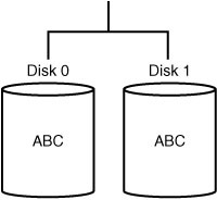
RAID 0: Stripe Set Without Parity

Although it’s given RAID status, RAID 0 does not actually provide any fault tolerance. In fact, using RAID 0 might even be less fault-tolerant than storing all your data on a single hard disk.

RAID 0 combines unused disk space on two or more hard drives into a single logical volume, with data written to equally sized stripes across all the disks. Using multiple disks, reads and writes are performed simultaneously across all drives. This means that disk access is faster, making the performance of RAID 0 better than other RAID solutions and significantly better than a single hard disk. The downside of RAID 0 is that if any disk in the array fails, the data is lost and must be restored from backup.

Because of its lack of fault tolerance, RAID 0 is rarely implemented. Figure 8.1 shows an example of RAID 0 striping across three hard disks.

FIGURE 8.1 RAID 0 striping without parity.

RAID 1

One of the more common RAID implementations is RAID 1. RAID 1 requires two hard disks and uses disk mirroring to provide fault tolerance. When information is written to the hard disk, it is automatically and simultaneously written to the second hard disk. Both of the hard disks in the mirrored configuration use the same hard disk controller; the partitions used on the hard disk need to be approximately the same size to establish the mirror. In the mirrored configuration, if the primary disk were to fail, the second mirrored disk would contain all the required information, and there would be little disruption to data availability. RAID 1 ensures that the server will continue operating in the case of primary disk failure.

A RAID 1 solution has some key advantages. First, it is cheap in terms of cost per megabyte of storage, because only two hard disks are required to provide fault tolerance. Second, no additional software is required to establish RAID 1, because modern network operating systems have built-in support for it. RAID levels using striping are often incapable of including a boot or system partition in fault tolerance solutions. Finally, RAID 1 offers load balancing over multiple disks, which increases read performance over that of a single disk. Write performance, however, is not improved.

Because of its advantages, RAID 1 is well suited as an entry-level RAID solution, but it has a few significant shortcomings that exclude its use in many environments. It has limited storage capacity—two 100GB hard drives provide only 100GB of storage space. Organizations with large data storage needs can exceed a mirrored solution capacity in very short order. RAID 1 also has a single point of failure, the hard disk controller. If it were to fail, the data would be inaccessible on either drive. Figure 8.2 shows an example of RAID 1 disk mirroring.

FIGURE 8.2 RAID 1 disk mirroring.

An extension of RAID 1 is disk duplexing. Disk duplexing is the same as mirroring, with the exception of one key detail: It places the hard disks on separate hard disk controllers, eliminating the single point of failure.

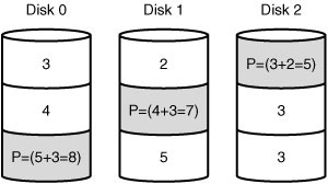
RAID 5

RAID 5, also known as disk striping with parity, uses distributed parity to write information across all disks in the array. Unlike the striping used in RAID 0, RAID 5 includes parity information in the striping, which provides fault tolerance. This parity information is used to re-create the data in the event of a failure. RAID 5 requires a minimum of three disks, with the equivalent of a single disk being used for the parity information. This means that if you have three 40GB hard disks, you have 80GB of storage space, with the other 40GB used for parity. To increase storage space in a RAID 5 array, you need only add another disk to the array. Depending on the sophistication of the RAID setup you are using, the RAID controller will be able to incorporate the new drive into the array automatically, or you will need to rebuild the array and restore the data from backup.

Many factors have made RAID 5 a very popular fault-tolerant design. RAID 5 can continue to function in the event of a single drive failure. If a hard disk in the array were to fail, the parity would re-create the missing data and continue to function with the remaining drives. The read performance of RAID 5 is improved over a single disk.

The RAID 5 solution has only a few drawbacks:

The costs of implementing RAID 5 are initially higher than other fault tolerance measures requiring a minimum of three hard disks. Given the costs of hard disks today, this is a minor concern. However, when it comes to implementing a RAID 5 solution, hardware RAID 5 is more expensive than a software-based RAID 5 solution.

RAID 5 suffers from poor write performance because the parity has to be calculated and then written across several disks. The performance lag is minimal and doesn’t have a noticeable difference on the network.

When a new disk is placed in a failed RAID 5 array, there is a regeneration time when the data is being rebuilt on the new drive. This process requires extensive resources from the server.

Figure 8.3 shows an example of RAID 5 striping with parity.

FIGURE 8.3 RAID 5 striping with parity.

RAID 10

Sometimes RAID levels are combined to take advantage of the best of each. One such strategy is RAID 10, which combines RAID levels 1 and 0. In this configuration, four disks are required. As you might expect, the configuration consists of a mirrored stripe set. To some extent, RAID 10 takes advantage of the performance capability of a stripe set while offering the fault tolerance of a mirrored solution. As well as having the benefits of each, though, RAID 10 inherits the shortcomings of each strategy. In this case, the high overhead and decreased write performance are the disadvantages. Figure 8.4 shows an example of a RAID 10 configuration. Table 8.2 summarizes the various RAID levels.

FIGURE 8.4 Disks in a RAID 10 configuration.

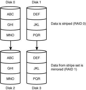
Table 8.2 Summary of RAID Levels

Server and Services Fault Tolerance

In addition to providing fault tolerance for individual hardware components, some organizations go the extra mile and include the entire server in the fault-tolerant design. Such a design keeps servers and the services they provide up and running. When it comes to server fault tolerance, two key strategies are commonly employed: standby servers and server clustering.

Standby Servers

Standby servers are a fault tolerance measure in which a second server is configured identically to the first one. The second server can be stored remotely or locally and set up in a failover configuration. In a failover configuration, the secondary server is connected to the primary and is ready to take over the server functions at a moment’s notice. If the secondary server detects that the primary has failed, it automatically cuts in. Network users will not notice the transition, because little or no disruption in data availability occurs.

The primary server communicates with the secondary server by issuing special notification notices called heartbeats. If the secondary server stops receiving the heartbeat messages, it assumes that the primary has died and therefore assumes the primary server configuration.

Server Clustering

Companies that want maximum data availability and that have the funds to pay for it can choose to use server clustering. As the name suggests, server clustering involves grouping servers for the purposes of fault tolerance and load balancing. In this configuration, other servers in the cluster can compensate for the failure of a single server. The failed server has no impact on the network, and the end users have no idea that a server has failed.

The clear advantage of server clusters is that they offer the highest level of fault tolerance and data availability. The disadvantage is equally clear—cost. The cost of buying a single server can be a huge investment for many organizations; having to buy duplicate servers is far too costly. In addition to just hardware costs, additional costs can be associated with recruiting administrators who have the skills to configure and maintain complex server clusters. Clustering provides the following advantages:

Increased performance: More servers equals more processing power. The servers in a cluster can provide levels of performance beyond the scope of a single system by combining resources and processing power.

Load balancing: Rather than having individual servers perform specific roles, a cluster can perform a number of roles, assigning the appropriate resources in the best places. This approach maximizes the power of the systems by allocating tasks based on which server in the cluster can best service the request.

Failover: Because the servers in the cluster are in constant contact with each other, they can detect and cope with the failure of an individual system. How transparent the failover is to users depends on the clustering software, the type of failure, and the capability of the application software being used to cope with the failure.

Scalability: The capability to add servers to the cluster offers a degree of scalability that is simply not possible in a single-server scenario. It is worth mentioning, though, that clustering on PC platforms is still in its relative infancy, and the number of machines that can be included in a cluster is still limited.

To make server clustering happen, you need certain ingredients—servers, storage devices, network links, and software that makes the cluster work.

Link Redundancy

Although a failed network card might not actually stop the server or a system, it might as well. A network server that cannot be used on the network results in server downtime. Although the chances of a failed network card are relatively low, attempts to reduce the occurrence of downtime have led to the development of a strategy that provides fault tolerance for network connections.

Through a process called adapter teaming, groups of network cards are configured to act as a single unit. The teaming capability is achieved through software, either as a function of the network card driver or through specific application software. The process of adapter teaming is not widely implemented; although the benefits it offers are many, so it’s likely to become a more common sight. The result of adapter teaming is increased bandwidth, fault tolerance, and the ability to manage network traffic more effectively. These features are broken into three sections:

Adapter fault tolerance: The basic configuration enables one network card to be configured as the primary device and others as secondary. If the primary adapter fails, one of the other cards can take its place without the need for intervention. When the original card is replaced, it resumes the role of primary controller.

Adapter load balancing: Because software controls the network adapters, workloads can be distributed evenly among the cards so that each link is used to a similar degree. This distribution allows for a more responsive server because one card is not overworked while another is underworked.

Link aggregation: This provides vastly improved performance by allowing more than one network card’s bandwidth to be aggregated—combined into a single connection. For example, through link aggregation, four 100Mbps network cards can provide a total of 400Mbps of bandwidth. Link aggregation requires that both the network adapters and the switch being used support it. In 1999, the IEEE ratified the 802.3ad standard for link aggregation, allowing compatible products to be produced.

Using Uninterruptible Power Supplies

No discussion of fault tolerance can be complete without a look at power-related issues and the mechanisms used to combat them. When you’re designing a fault-tolerant system, your planning should definitely include uninterruptible power supplies (UPSs). A UPS serves many functions and is a major part of server consideration and implementation.

On a basic level, a UPS is a box that holds a battery and built-in charging circuit. During times of good power, the battery is recharged; when the UPS is needed, it’s ready to provide power to the server. Most often, the UPS is required to provide enough power to give the administrator time to shut down the server in an orderly fashion, preventing any potential data loss from a dirty shutdown.

Why Use a UPS?

Organizations of all shapes and sizes need UPSs as part of their fault tolerance strategies. A UPS is as important as any other fault tolerance measure. Three key reasons make a UPS necessary:

Data availability: The goal of any fault tolerance measure is data availability. A UPS ensures access to the server in the event of a power failure—or at least as long as it takes to save a file.

Protection from data loss: Fluctuations in power or a sudden power-down can damage the data on the server system. In addition, many servers take full advantage of caching, and a sudden loss of power could cause the loss of all information held in cache.

Protection from hardware damage: Constant power fluctuations or sudden power-downs can damage hardware components within a computer. Damaged hardware can lead to reduced data availability while the hardware is being repaired.

Power Threats

In addition to keeping a server functioning long enough to safely shut it down, a UPS safeguards a server from inconsistent power. This inconsistent power can take many forms. A UPS protects a system from the following power-related threats:

Blackout: A total failure of the power supplied to the server.

Spike: A spike is a very short (usually less than a second) but very intense increase in voltage. Spikes can do irreparable damage to any kind of equipment, especially computers.

Surge: Compared to a spike, a surge is a considerably longer (sometimes many seconds) but usually less intense increase in power. Surges can also damage your computer equipment.

Sag: A sag is a short-term voltage drop (the opposite of a spike). This type of voltage drop can cause a server to reboot.

Brownout: A brownout is a drop in voltage that usually lasts more than a few minutes.

Many of these power-related threats can occur without your knowledge; if you don’t have a UPS, you cannot prepare for them. For the cost, it is worth buying a UPS, if for no other reason than to sleep better at night.

Disaster Recovery

Even the most fault-tolerant networks will fail, which is an unfortunate fact. When those costly and carefully implemented fault tolerance strategies fail, you are left with disaster recovery.

Disaster recovery can take many forms. In addition to disasters such as fire, flood, and theft, many other potential business disruptions can fall under the banner of disaster recovery. For example, the failure of the electrical supply to your city block might interrupt the business functions. Such an event, although not a disaster per se, might invoke the disaster recovery methods.

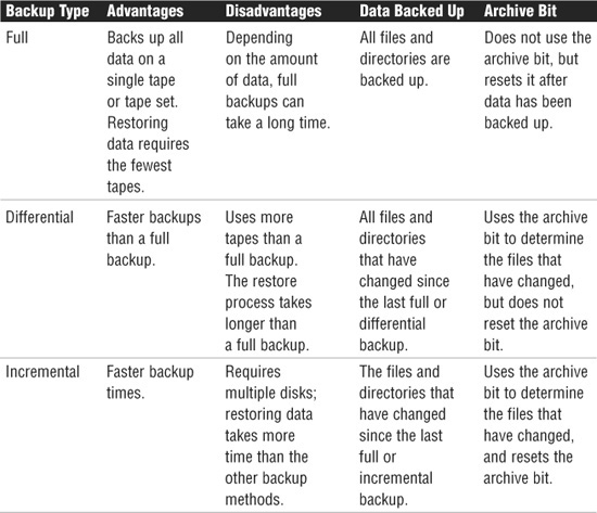
The cornerstone of every disaster recovery strategy is the preservation and recoverability of data. When talking about preservation and recoverability, we are talking about backups. When we are talking about backups, we are likely talking about tape backups. Implementing a regular backup schedule can save you a lot of grief when fault tolerance fails or when you need to recover a file that has been accidentally deleted. When it comes time to design a backup schedule, three key types of backups are used—full, differential, and incremental.

Full Backup

The preferred method of backup is the full backup method, which copies all files and directories from the hard disk to the backup media. There are a few reasons why doing a full backup is not always possible. First among them is likely the time involved in performing a full backup.

Depending on the amount of data to be backed up, full backups can take an extremely long time and can use extensive system resources. Depending on the configuration of the backup hardware, this can slow down the network considerably. In addition, some environments have more data than can fit on a single tape. This makes doing a full backup awkward, because someone might need to be there to change the tapes.

The main advantage of full backups is that a single tape or tape set holds all the data you need backed up. In the event of a failure, a single tape might be all that is needed to get all data and system information back. The upshot of all this is that any disruption to the network is greatly reduced.

Unfortunately, its strength can also be its weakness. A single tape holding an organization’s data can be a security risk. If the tape were to fall into the wrong hands, all the data could be restored on another computer. Using passwords on tape backups and using a secure offsite and onsite location can minimize the security risk.

Differential Backup

Companies that just don’t have enough time to complete a full backup daily can make use of the differential backup. Differential backups are faster than a full backup, because they back up only the data that has changed since the last full backup. This means that if you do a full backup on a Saturday and a differential backup on the following Wednesday, only the data that has changed since Saturday is backed up. Restoring the differential backup requires the last full backup and the latest differential backup.

Differential backups know what files have changed since the last full backup because they use a setting called the archive bit. The archive bit flags files that have changed or have been created and identifies them as ones that need to be backed up. Full backups do not concern themselves with the archive bit, because all files are backed up, regardless of date. A full backup, however, does clear the archive bit after data has been backed up to avoid future confusion. Differential backups take notice of the archive bit and use it to determine which files have changed. The differential backup does not reset the archive bit information.

Incremental Backup

Some companies have a finite amount of time they can allocate to backup procedures. Such organizations are likely to use incremental backups in their backup strategy. Incremental backups save only the files that have changed since the last full or incremental backup. Like differential backups, incremental backups use the archive bit to determine which files have changed since the last full or incremental backup. Unlike differentials, however, incremental backups clear the archive bit, so files that have not changed are not backed up.

The faster backup time of incremental backups comes at a price—the amount of time required to restore. Recovering from a failure with incremental backups requires numerous tapes—all the incremental tapes and the most recent full backup. For example, if you had a full backup from Sunday and an incremental for Monday, Tuesday, and Wednesday, you would need four tapes to restore the data. Keep in mind that each tape in the rotation is an additional step in the restore process and an additional failure point. One damaged incremental tape, and you will be unable to restore the data. Table 8.3 summarizes the various backup strategies.

Table 8.3 Backup Strategies

Tape Rotations

After you select a backup type, you are ready to choose a backup rotation. Several backup rotation strategies are in use—some good, some bad, and some really bad. The most common, and perhaps the best, rotation strategy is grandfather, father, son (GFS).

The GFS backup rotation is the most widely used—and for good reason. For example, a GFS rotation may require 12 tapes: four tapes for daily backups (son), five tapes for weekly backups (father), and three tapes for monthly backups (grandfather).

Using this rotation schedule, you can recover data from days, weeks, or months earlier. Some network administrators choose to add tapes to the monthly rotation so that they can retrieve data even further back, sometimes up to a year. In most organizations, however, data that is a week old is out of date, let alone six months or a year.

Backup Best Practices

Many details go into making a backup strategy a success. The following are issues to consider as part of your backup plan:

Offsite storage: Consider storing backup tapes offsite so that in the event of a disaster in a building, a current set of tapes is still available offsite. The offsite tapes should be as current as any onsite and should be secure.

Label tapes: The goal is to restore the data as quickly as possible, and trying to find the tape you need can be difficult if it isn’t marked. Furthermore, this can prevent you from recording over a tape you need.

New tapes: Like old cassette tapes, the tape cartridges used for the backups wear out over time. One strategy used to prevent this from becoming a problem is to periodically introduce new tapes into the rotation schedule.

Verify backups: Never assume that the backup was successful. Seasoned administrators know that checking backup logs and performing periodic test restores are part of the backup process.

Cleaning: You need to clean the tape drive occasionally. If the inside gets dirty, backups can fail.

Hot and Cold Spares

The impact that a failed component has on a system or network depends largely on the predisaster preparation and on the recovery strategies used. Hot and cold spares represent a strategy for recovering from failed components.

Hot Spares and Hot Swapping

Hot spares allow system administrators to quickly recover from component failure. In a common use, a hot spare enables a RAID system to automatically fail over to a spare hard drive should one of the other drives in the RAID array fail. A hot spare does not require any manual intervention. Instead, a redundant drive resides in the system at all times, just waiting to take over if another drive fails. The hot spare drive takes over automatically, leaving the failed drive to be removed later. Even though hot-spare technology adds an extra level of protection to your system, after a drive has failed and the hot spare has been used, the situation should be remedied as soon as possible.

Hot swapping is the ability to replace a failed component while the system is running. Perhaps the most commonly identified hot-swap component is the hard drive. In certain RAID configurations, when a hard drive crashes, hot swapping allows you to simply take the failed drive out of the server and install a new one.

The benefits of hot swapping are very clear in that it allows a failed component to be recognized and replaced without compromising system availability. Depending on the system’s configuration, the new hardware normally is recognized automatically by both the current hardware and the operating system. Nowadays, most internal and external RAID subsystems support the hot-swapping feature. Some hot-swappable components include power supplies and hard disks.

Cold Spares and Cold Swapping

The term cold spare refers to a component, such as a hard disk, that resides within a computer system but requires manual intervention in case of component failure. A hot spare engages automatically, but a cold spare might require configuration settings or some other action to engage it. A cold spare configuration typically requires a reboot of the system.

The term cold spare has also been used to refer to a redundant component that is stored outside the actual system but is kept in case of component failure. To replace the failed component with a cold spare, you need to power down the system.

Cold swapping refers to replacing components only after the system is completely powered off. This strategy is by far the least attractive for servers, because the services provided by the server are unavailable for the duration of the cold-swap procedure. Modern systems have come a long way to ensure that cold swapping is a rare occurrence. For some situations and for some components, however, cold swapping is the only method to replace a failed component. The only real defense against having to shut down the server is to have redundant components reside in the system.

Hot, Warm, and Cold Sites

A disaster recovery plan might include the provision for a recovery site that can be brought into play quickly. These sites fall into three categories: hot, warm, and cold. The need for each of these types of sites depends largely on the business you are in and the funds available. Disaster recovery sites represent the ultimate in precautions for organizations that really need them. As a result, they don’t come cheap.

The basic concept of a disaster recovery site is that it can provide a base from which the company can be operated during a disaster. The disaster recovery site normally is not intended to provide a desk for every employee. It’s intended more as a means to allow key personnel to continue the core business functions.

In general, a cold recovery site is a site that can be up and operational in a relatively short amount of time, such as a day or two. Provision of services, such as telephone lines and power, is taken care of, and the basic office furniture might be in place. But there is unlikely to be any computer equipment, even though the building might well have a network infrastructure and a room ready to act as a server room. In most cases, cold sites provide the physical location and basic services.

Cold sites are useful if you have some forewarning of a potential problem. Generally speaking, cold sites are used by organizations that can weather the storm for a day or two before they get back up and running. If you are the regional office of a major company, it might be possible to have one of the other divisions take care of business until you are ready to go. But if you are the one and only office in the company, you might need something a little hotter.

For organizations with the dollars and the desire, hot recovery sites represent the ultimate in fault tolerance strategies. Like cold recovery sites, hot sites are designed to provide only enough facilities to continue the core business function, but hot recovery sites are set up to be ready to go at a moment’s notice.

A hot recovery site includes phone systems with the phone lines already connected. Data networks also are in place, with any necessary routers and switches plugged in and turned on. Desks have desktop PCs installed and waiting, and server areas are replete with the necessary hardware to support business-critical functions. In other words, within a few hours, the hot site can become a fully functioning element of an organization.

The issue that confronts potential hot-recovery site users is simply that of cost. Office space is expensive in the best of times, but having space sitting idle 99.9 percent of the time can seem like a tremendously poor use of money. A very popular strategy to get around this problem is to use space provided in a disaster recovery facility, which is basically a building, maintained by a third-party company, in which various businesses rent space. Space is usually apportioned according to how much each company pays.

Sitting between the hot and cold recovery sites is the warm site. A warm site typically has computers but is not configured ready to go. This means that data might need to be upgraded or other manual interventions might need to be performed before the network is again operational. The time it takes to get a warm site operational lands right in the middle of the other two options, as does the cost.

Network Optimization Strategies

Today’s networks are all about speed. Network users expect data and application delivery quickly. Just look at how impatient many of us get waiting for web pages to load. Networks, however, are saturated and congested with traffic, making it necessary to have strategies to ensure that we are using bandwidth in the best possible way. These strategies are collectively referred to as quality of service (QoS).

QoS

QoS describes the strategies used to manage and increase the flow of network traffic. QoS features allow administrators to predict bandwidth use, monitor that use, and control it to ensure that bandwidth is available to the applications that need it. These applications generally can be broken into two categories:

Latency-sensitive: These applications need bandwidth for quick delivery where network lag time impacts their effectiveness. This includes voice and video transfer. For example, voice over IP (VoIP) would be difficult to use if there were a significant lag time in the conversation.

Latency-insensitive: Controlling bandwidth also involves managing latency-insensitive applications. This includes bulk data transfers such as huge backup procedures and File Transfer Protocol (FTP) transfers.

With bandwidth being limited, and networks becoming increasingly congested, it becomes more difficult to deliver latency-sensitive traffic. If network traffic continues to increase and we can’t always increase bandwidth, the choice is to prioritize traffic to ensure timely delivery. This is where QoS really comes into play. QoS ensures the delivery of applications, such as videoconferencing and VoIP telephony, without adversely affecting network throughput. QoS achieves more efficient use of network resources by differentiating between latency-insensitive traffic such as fax data and latency-sensitive streaming media.

One important strategy for QoS is priority queuing. Essentially what happens is that traffic is placed in order based on its importance on delivery time. All data is given access, but the more important and latency-sensitive data is given higher priority.

Traffic Shaping

Traffic shaping is a QoS strategy that is designed to enforce prioritization policies on the transmission of data throughout the network. It is intended to reduce latency by controlling the amount of data that flows into and out of the network. Traffic is categorized, queued, and directed according to network policies.

Methods Used for Traffic Shaping

You can shape and limit network traffic using several different strategies. Which one you choose depends on the network’s needs and the amount of traffic. Here are some common traffic-shaping methods:

Shaping by application: Administrators can configure a traffic shaper by categorizing specific types of network traffic and assigning that category a bandwidth limit. For example, traffic can be categorized using FTP. The rule can specify that no more than 4Mbps be dedicated for FTP traffic. This same principle can apply to Telnet sessions, streaming audio, or any other application coming through the network.

Shaping network traffic per user: Every network has users who use more bandwidth than others. Some of this might be work-related, but more often than not, it is personal use. In such a case, it may be necessary to establish traffic shaping on a per-user basis. Traffic shapers allow administrators to delegate a certain bandwidth to a user. For instance, Bob from accounting is allowed no more than 256Kbps. This doesn’t limit what the user can access, just the speed at which that content can be accessed.

Priority shaping: One important consideration when looking at traffic shaping is determining which traffic is mission-critical and which is less so. In addition to setting hard or burstable traffic limits on a per-application or per-user basis, traffic shaping devices can also be used to define the relative importance, or priority, of different types of traffic. For example, in an academic network where teaching and research are most important, recreational uses of the network (such as network games or peer-to-peer file-sharing application traffic) can be allowed bandwidth only when higher-priority applications don’t need it.

Caching Engines

Caching is an important consideration when optimizing network traffic. For example, as discussed in Chapter 3, “Networking Components and Devices,” proxy servers use caching to limit the number of client requests that go to the Internet. Instead, the requests are filled from the proxy server’s cache. Recall from Chapter 3 that when a caching proxy server has answered a request for a web page, the server makes a copy of all or part of that page in its cache. Then, when the page is requested again, the proxy server answers the request from the cache rather than going back out to the Internet. For example, if a client on a network requests the web page www.comptia.org, the proxy server can cache the contents of that web page. When a second client computer on the network attempts to access the same site, that client can grab it from the proxy server cache; accessing the Internet is not necessary. This greatly reduces the network traffic that has to be filtered to the Internet, a significant gain in terms of network optimization.

When it comes to determining what to cache, an administrator can establish many rules:

What websites to cache

How long the information is cached

When cached information is updated

The size of cached information

What type of content is cached

Who can access the cache

The rules for caching vary from network to network, depending on the network’s needs. In networks where a large number of people access similar websites, caching can greatly increase network performance. The advantages of properly configured caching are clear—reduced bandwidth, and latency and increased throughput. One possible disadvantage of caching is receiving out-of-date files, because you are obtaining content from the caching engine and not the website itself.

Working with Command-Line Utilities

For anyone working with TCP/IP networks, troubleshooting connectivity is something that simply must be done. This section describes the tools that are used in the troubleshooting process and identifies scenarios in which they can be used.

Troubleshooting with Diagnostic Utilities

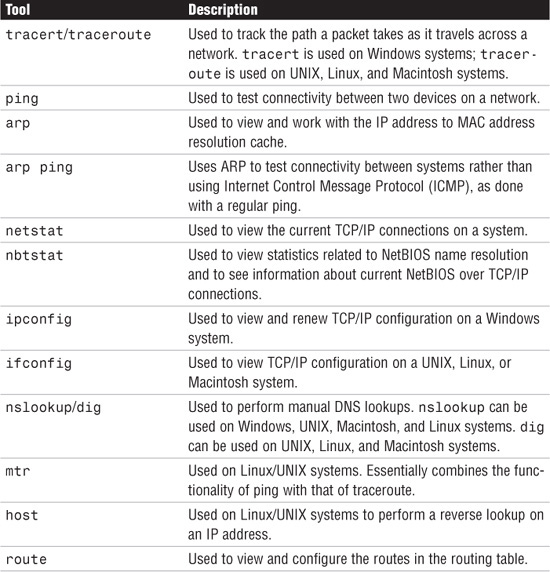
You can use many utilities when troubleshooting TCP/IP. Although the actual utilities available vary from platform to platform, the functionality between platforms is quite similar. Table 8.4 lists the TCP/IP troubleshooting tools covered on the Network+ exam, along with their purpose.

Table 8.4 Common TCP/IP Troubleshooting Tools and Their Purposes

The following sections look in more detail at these utilities and the output they produce.

The Trace Route Utility (tracert/traceroute)

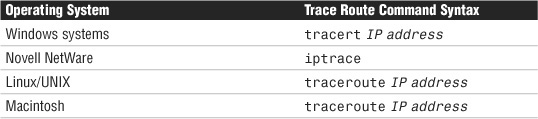
The trace route utility does exactly what its name implies—it traces the route between two hosts. It does this by using ICMP echo packets to report information at every step in the journey. Each of the common network operating systems provides a trace route utility, but the name of the command and the output vary slightly on each. However, for the purposes of the Network+ exam, you should not concern yourself with the minor differences in the output format. Table 8.5 shows the trace route command syntax used in various operating systems.

Table 8.5 Trace Route Utility Commands

Trace route provides a lot of useful information, including the IP address of every router connection it passes through and, in many cases, the name of the router (although this depends on the router’s configuration). Trace route also reports the length, in milliseconds, of the round-trip the packet made from the source location to the router and back. This information can help identify where network bottlenecks or breakdowns might be. The following is an example of a successful tracert command on a Windows Server system:

Similar to the other common operating systems covered on the Network+ exam, the tracert display on a Windows-based system includes several columns of information. The first column represents the hop number. You may recall that hop is the term used to describe a step in the path a packet takes as it crosses the network. The next three columns indicate the round-trip time, in milliseconds, that a packet takes in its attempts to reach the destination. The last column is the hostname and the IP address of the responding device.

Of course, not all trace route attempts are successful. The following is the output from a tracert command on a Windows Server system that doesn’t manage to get to the remote host:

C:>tracert comptia.org

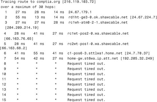
In this example, the trace route request gets to only the seventh hop, at which point it fails. This failure indicates that the problem lies on the far side of the device in step 7 or on the near side of the device in step 8. In other words, the device at step 7 is functioning but might not be able to make the next hop. The cause of the problem could be a range of things, such as an error in the routing table or a faulty connection. Alternatively, the seventh device might be operating at 100 percent, but device 8 might not be functioning at all. In any case, you can isolate the problem to just one or two devices.

The trace route utility can also help you isolate a heavily congested network. In the following example, the trace route packets fail in the midst of the tracert from a Windows Server system, but subsequently they continue. This behavior can be an indicator of network congestion:

C:>tracert comptia.org

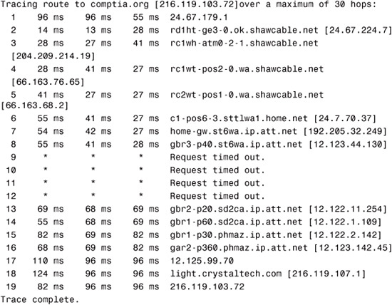
Generally speaking, trace route utilities allow you to identify the location of a problem in the connectivity between two devices. After you have determined this location, you might need to use a utility such as ping to continue troubleshooting. In many cases, as in the examples provided in this chapter, the routers might be on a network such as the Internet and therefore not within your control. In that case, you can do little except inform your ISP of the problem.

ping

Most network administrators are very familiar with the ping utility and are likely to use it on an almost daily basis. The basic function of the ping command is to test the connectivity between the two devices on a network. All the command is designed to do is determine whether the two computers can see each other and to notify you of how long the round-trip takes to complete.

Although ping is most often used on its own, a number of switches can be used to assist in the troubleshooting process. Table 8.6 shows some of the commonly used switches with ping on a Windows system.

Table 8.6 ping Command Switches

ping works by sending ICMP echo request messages to another device on the network. If the other device on the network hears the ping request, it automatically responds with an ICMP echo reply. By default, the ping command on a Windows-based system sends four data packets; however, using the -t switch, a continuous stream of ping requests can be sent.

ping is perhaps the most widely used of all network tools; it is primarily used to verify connectivity between two network devices. On a good day, the results from the ping command are successful, and the sending device receives a reply from the remote device. Not all ping results are that successful. To be able to use ping effectively, you must be able to interpret the results of a failed ping command.

The Destination Host Unreachable Message

The Destination host unreachable error message means that a route to the destination computer system cannot be found. To remedy this problem, you might need to examine the routing information on the local host to confirm that the local host is correctly configured, or you might need to make sure that the default gateway information is correct. The following is an example of a ping failure that gives the Destination host unreachable message:

Pinging 24.67.54.233 with 32 bytes of data: Destination host unreachable.

Destination host unreachable.

Destination host unreachable.

Destination host unreachable.

Ping statistics for 24.67.54.233:

Packets: Sent = 4, Received = 0, Lost = 4 (100% loss), Approximate round trip times in milli-seconds:

Minimum = 0ms, Maximum = 0ms, Average = 0ms

The Request Timed Out Message

The Request timed out error message is very common when you use the ping command. Essentially, this error message indicates that your host did not receive the ping message back from the destination device within the designated time period. Assuming that the network connectivity is okay on your system, this typically indicates that the destination device is not connected to the network, is powered off, or is not configured correctly. It could also mean that some intermediate device is not operating correctly. In some rare cases, it can also indicate that the network has so much congestion that timely delivery of the ping message could not be completed. It might also mean that the ping is being sent to an invalid IP address or that the system is not on the same network as the remote host, and an intermediary device is not configured correctly. In any of these cases, the failed ping should initiate a troubleshooting process that might involve other tools, manual inspection, and possibly reconfiguration. The following example shows the output from a ping to an invalid IP address:

C:>ping 169.76.54.3
Pinging 169.76.54.3 with 32 bytes of data:

Request timed out.
Request timed out.
Request timed out.
Request timed out.

Ping statistics for 169.76.54.3:
      Packets: Sent = 4, Received = 0, Lost = 4 (100%
Approximate round trip times in milli-seconds:
      Minimum = 0ms, Maximum = 0ms, Average = 0ms

During the ping request, you might receive some replies from the remote host that are intermixed with Request timed out errors. This is often the result of a congested network. An example follows; notice that this example, which was run on a Windows Vista system, uses the -t switch to generate continuous pings:

C:>ping -t 24.67.184.65
Pinging 24.67.184.65 with 32 bytes of data:

Reply from 24.67.184.65: bytes=32 time=55ms TTL=127
Reply from 24.67.184.65: bytes=32 time=54ms TTL=127
Reply from 24.67.184.65: bytes=32 time=27ms TTL=127
Request timed out.
Request timed out.
Request timed out.
Reply from 24.67.184.65: bytes=32 time=69ms TTL=127
Reply from 24.67.184.65: bytes=32 time=28ms TTL=127
Reply from 24.67.184.65: bytes=32 time=28ms TTL=127
Reply from 24.67.184.65: bytes=32 time=68ms TTL=127
Reply from 24.67.184.65: bytes=32 time=41ms TTL=127
Ping statistics for 24.67.184.65:
      Packets: Sent = 11, Received = 8, Lost = 3 (27% loss),
Approximate round trip times in milli-seconds:
      Minimum = 27ms, Maximum = 69ms, Average = 33ms

In this example, three packets were lost. If this continued on your network, you would need to troubleshoot to find out why packets were being dropped.

The Unknown Host Message

The Unknown host error message is generated when the hostname of the destination computer cannot be resolved. This error usually occurs when you ping an incorrect hostname, as shown in the following example, or try to use ping with a hostname when hostname resolution (via DNS or a HOSTS text file) is not configured:

C:>ping www.comptia.ca

Unknown host www.comptia.ca

If the ping fails, you need to verify that the ping is being sent to the correct remote host. If it is, and if name resolution is configured, you have to dig a little more to find the problem. This error might indicate a problem with the name resolution process, and you might need to verify that the DNS or WINS server is available. Other commands, such as nslookup or dig, can help in this process.

The Expired TTL Message

The Time to Live (TTL) is an important consideration in understanding the ping command. The function of the TTL is to prevent circular routing, which occurs when a ping request keeps looping through a series of hosts. The TTL counts each hop along the way toward its destination device. Each time it counts one hop, the hop is subtracted from the TTL. If the TTL reaches 0, it has expired, and you get a message like the following:

Reply from 24.67.180.1: TTL expired in transit

If the TTL is exceeded with ping, you might have a routing problem on the network. You can modify the TTL for ping on a Windows system by using the ping -i command.

Troubleshooting with ping

Although ping does not completely isolate problems, you can use it to help identify where a problem lies. When troubleshooting with ping, follow these steps:

1. Ping the IP address of your local loopback using the command ping 127.0.0.1. If this command is successful, you know that the TCP/IP protocol suite is installed correctly on your system and is functioning. If you are unable to ping the local loopback adapter, TCP/IP might need to be reloaded or reconfigured on the machine you are using.

2. Ping the assigned IP address of your local network interface card (NIC). If the ping is successful, you know that your NIC is functioning on the network and has TCP/IP correctly installed. If you are unable to ping the local NIC, TCP/IP might not be bound to the NIC correctly, or the NIC drivers might be improperly installed.

3. Ping the IP address of another known good system on your local network. By doing so, you can determine whether the computer you are using can see other computers on the network. If you can ping other devices on your local network, you have network connectivity.

If you cannot ping other devices on your local network, but you could ping the IP address of your system, you might not be connected to the network correctly.

4. After you’ve confirmed that you have network connectivity for the local network, you can verify connectivity to a remote network by sending a ping to the IP address of the default gateway.

5. If you can ping the default gateway, you can verify remote connectivity by sending a ping to the IP address of a system on a remote network.

Using just the ping command in these steps, you can confirm network connectivity on not only the local network, but also on a remote network. The whole process requires as much time as it takes to enter the command, and you can do it all from a single location.

If you are an optimistic person, you can perform step 5 first. If that works, all the other steps will also work, saving you the need to test them. If your step 5 trial fails, you can go to step 1 and start the troubleshooting process from the beginning.

ARP

Address Resolution Protocol (ARP) is used to resolve IP addresses to MAC addresses. This is important because on a network, devices find each other using the IP address, but communication between devices requires the MAC address.

When a computer wants to send data to another computer on the network, it must know the MAC address (physical address) of the destination system. To discover this information, ARP sends out a discovery packet to obtain the MAC address. When the destination computer is found, it sends its MAC address to the sending computer. The ARP-resolved MAC addresses are stored temporarily on a computer system in the ARP cache. Inside this ARP cache is a list of matching MAC and IP addresses. This ARP cache is checked before a discovery packet is sent to the network to determine if there is an existing entry.

Entries in the ARP cache are periodically flushed so that the cache doesn’t fill up with unused entries. The following code shows an example of the arp command with the output from a Windows server system:

C:>arp -a
Interface: 24.67.179.22 on Interface 0x3

As you might notice, the type is listed as dynamic. Entries in the ARP cache can be added statically or dynamically. Static entries are added manually and do not expire. The dynamic entries are added automatically when the system accesses another on the network.

As with other command-line utilities, several switches are available for the arp command. Table 8.7 shows the available switches for Windows-based systems.

Table 8.7 arp Switches

arp ping

Earlier in this chapter we talked about the ping command and how it is used to test connectivity between devices on a network. Using the ping command is often an administrator’s first step to test connectivity between network devices. If the ping fails, it is assumed that the device you are pinging is offline. But this may not always be the case.

Most companies now use firewalls or other security measures that may block ICMP requests. This means that a ping request will not work. Blocking ICMP is a security measure; if a would-be hacker cannot hit the target, he may not attack the host.

If ICMP is blocked, you have still another option to test connectivity with a device on the network—the arp ping. As mentioned, the ARP utility is used to resolve IP addresses to MAC addresses. The arp ping utility does not use the ICMP protocol to test connectivity like ping does, rather it uses the ARP protocol. However, ARP is not routable, and the arp ping cannot be routed to work over separate networks. The arp ping works only on the local subnet.

Just like with a regular ping, an arp ping specifies an IP address; however, instead of returning regular ping results, the arp ping responds with the MAC address and name of the computer system. So, when a regular ping using ICMP fails to locate a system, the arp ping uses a different method to find the system. With arp ping, it is possible to ping a MAC address directly. From this, it is possible to determine if duplicate IP addresses are used and, as mentioned, determine if a system is responding.

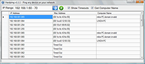
arp ping is not built into Windows, but you can download a number of programs that allow you to ping using ARP. Linux, on the other hand, has an arp ping utility ready to use. Figure 8.5 shows the results of an arp ping from a shareware Windows utility.

FIGURE 8.5 An example of an arp ping.

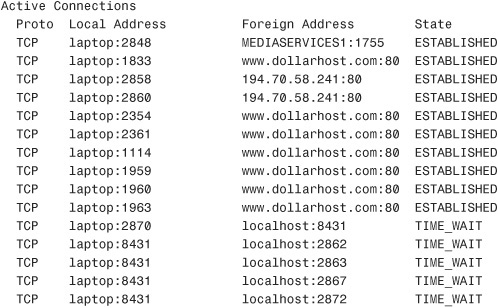
The netstat Command

The netstat command displays the protocol statistics and current TCP/IP connections on the local system. Used without any switches, the netstat command shows the active connections for all outbound TCP/IP connections. In addition, several switches are available that change the type of information netstat displays. Table 8.8 shows the various switches available for the netstat utility.

Table 8.8 netstat Switches

The netstat utility is used to show the port activity for both TCP and UDP connections, showing the inbound and outbound connections. When used without switches, the netstat utility has four information headings.

Proto: Lists the protocol being used, either UDP or TCP.

Local address: Specifies the local address and port being used.

Foreign address: Identifies the destination address and port being used.

State: Specifies whether the connection is established.

In its default usage, the netstat command shows outbound connections that have been established by TCP. The following shows sample output from a netstat command without using any switches:

C:>netstat

As with any other command-line utility, the netstat utility has a number of switches. The following sections briefly explain the switches and give sample output from each.

netstat -e

The netstat -e command shows the activity for the NIC and displays the number of packets that have been both sent and received. Here’s an example:

C:WINDOWSDesktop>netstat -e
Interface Statistics

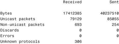
As you can see, the netstat -e command shows more than just the packets that have been sent and received:

Bytes: The number of bytes that the NIC has sent or received since the computer was turned on.

Unicast packets: Packets sent and received directly by this interface.

Non-unicast packets: Broadcast or multicast packets that the NIC picked up.

Discards: The number of packets rejected by the NIC, perhaps because they were damaged.

Errors: The errors that occurred during either the sending or receiving process. As you would expect, this column should be a low number. If it is not, this could indicate a problem with the NIC.

Unknown protocols: The number of packets that the system could not recognize.

netstat -a

The netstat -a command displays statistics for both TCP and User Datagram Protocol (UDP). Here is an example of the netstat -a command:

As you can see, the output includes four columns, which show the protocol, the local address, the foreign address, and the port’s state. The TCP connections show the local and foreign destination addresses and the connection’s current state. UDP, however, is a little different. It does not list a state status because, as mentioned throughout this book, UDP is a connectionless protocol and does not establish connections. The following list briefly explains the information provided by the netstat -a command:

Proto: The protocol used by the connection.

Local Address: The IP address of the local computer system and the port number it is using. If the entry in the local address field is an asterisk (*), the port has not yet been established.

Foreign Address: The IP address of a remote computer system and the associated port. When a port has not been established, as with the UDP connections, *:* appears in the column.

State: The current state of the TCP connection. Possible states include established, listening, closed, and waiting.

netstat -r

The netstat -r command is often used to view a system’s routing table. A system uses a routing table to determine routing information for TCP/IP traffic. The following is an example of the netstat -r command from a Windows Vista system:

C:WINDOWSDesktop>netstat -r

Route table

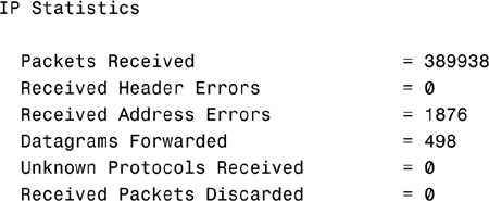
netstat -s

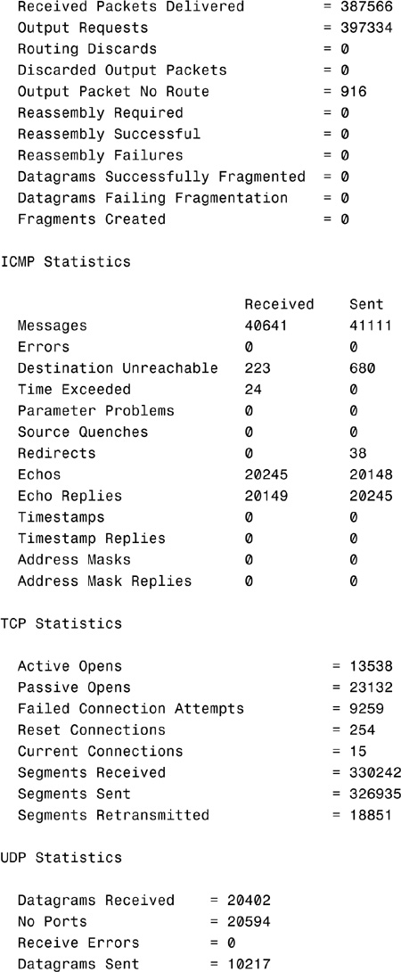
The netstat -s command displays a number of statistics related to the TCP/IP protocol suite. Understanding the purpose of every field in the output is beyond the scope of the Network+ exam, but for your reference, sample output from the netstat -s command is shown here:

nbtstat

The nbtstat utility is used to view protocol statistics and information for NetBIOS over TCP/IP connections. nbtstat is commonly used to troubleshoot NetBIOS name resolution problems. Because nbtstat resolves NetBIOS names, it’s available only on Windows systems.

A number of case-sensitive switches are available for the nbtstat command, as shown in Table 8.9.

Table 8.9 nbtstat Switches

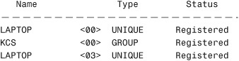
For example, the following is the output from the nbtstat -n command:

C:>nbtstat -n
Lana # 0:
Node IpAddress: [169.254.196.192] Scope Id: []
NetBIOS Local Name Table

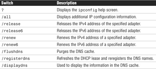
The ipconfig Command

The ipconfig command is a technician’s best friend when it comes to viewing the TCP/IP configuration of a Windows system. Used on its own, the ipconfig command shows basic information such as the name of the local network interface, the IP address, the subnet mask, and the default gateway. Combined with the /all switch, it shows a detailed set of information, as shown in the following example:

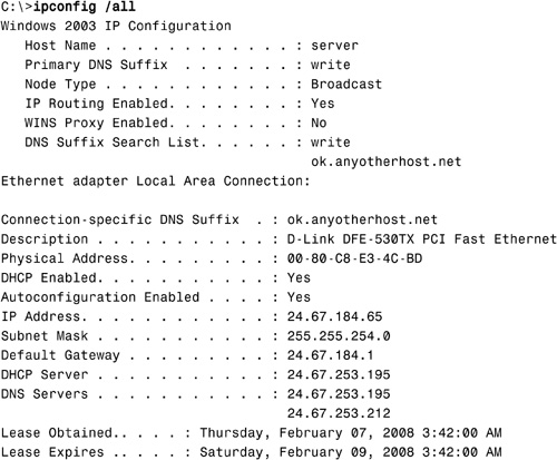
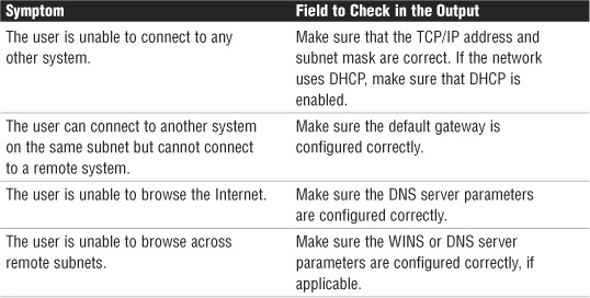
As you can imagine, you can use the output from the ipconfig /all command in a massive range of troubleshooting scenarios. Table 8.10 lists some of the most common troubleshooting symptoms, along with where to look for clues about solving them in the ipconfig /all output.

Table 8.10 Common Troubleshooting Symptoms That ipconfig Can Help Solve

Using the /all switch might be far and away the most popular, but there are a few others. These include the switches listed in Table 8.11.

Table 8.11 ipconfig Switches

ifconfig

ifconfig performs the same function as ipconfig, but on a Linux, UNIX, or Macintosh system. Because Linux relies more heavily on command-line utilities than Windows, the Linux and UNIX version of ifconfig provides much more functionality than ipconfig. On a Linux or UNIX system, you can get information about the usage of the ifconfig command by using ifconfig --help. The following output provides an example of the basic ifconfig command run on a Linux system:

Although the ifconfig command displays the IP address, subnet mask, and default gateway information for both the installed network adapter and the local loopback adapter, it does not report DHCP lease information. Instead, you can use the pump -s command to view detailed information on the DHCP lease, including the assigned IP address, the address of the DHCP server, and the time remaining on the lease. The pump command can also be used to release and renew IP addresses assigned via DHCP and to view DNS server information.

nslookup

nslookup is a utility used to troubleshoot DNS-related problems. Using nslookup, you can, for example, run manual name resolution queries against DNS servers, get information about your system’s DNS configuration, or specify what kind of DNS record should be resolved.

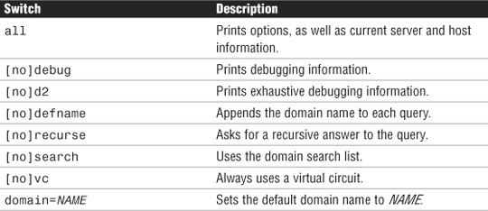
When nslookup is started, it displays the current hostname and the IP address of the locally configured DNS server. You then see a command prompt that allows you to specify further queries. This is known as interactive mode. Table 8.12 lists the commands you can enter in interactive mode.

Table 8.12 nslookup Switches

Instead of using interactive mode, you can also execute nslookup requests directly at the command prompt. The following listing shows the output from the nslookup command when a domain name is specified to be resolved:

C:>nslookup comptia.org
Server: nsc1.ht.ok.shawcable.net
Address: 64.59.168.13
Non-authoritative answer:
Name: comptia.org
Address: 208.252.144.4

As you can see from the output, nslookup shows the hostname and IP address of the DNS server against which the resolution was performed, along with the hostname and IP address of the resolved host.

dig

dig is used on a Linux, UNIX, or Macintosh system to perform manual DNS lookups. dig performs the same basic task as nslookup, but with one major distinction: The dig command does not have an interactive mode and instead uses only command-line switches to customize results.

dig generally is considered a more powerful tool than nslookup, but in the course of a typical network administrator’s day, the minor limitations of nslookup are unlikely to be too much of a factor. Instead, dig is often simply the tool of choice for DNS information and troubleshooting on UNIX, Linux, or Macintosh systems. Like nslookup, dig can be used to perform simple name resolution requests. The output from this process is shown in the following listing:

As you can see, dig provides a number of pieces of information in the basic output—more so than nslookup. Network administrators can gain information from three key areas of the output—ANSWER SECTION, AUTHORITY SECTION, and the last four lines of the output.

The ANSWER SECTION of the output provides the name of the domain or host being resolved, along with its IP address. The A in the results line indicates the record type that is being resolved.

The AUTHORITY SECTION provides information on the authoritative DNS servers for the domain against which the resolution request was performed. This information can be useful in determining whether the correct DNS servers are considered authoritative for a domain.

The last four lines of the output show how long the name resolution request took to process and the IP address of the DNS server that performed the resolution. It also shows the date and time of the request, as well as the size of the packets sent and received.

mtr

The My traceroute (mtr) command is used on Linux/UNIX systems. Essentially it combines the functionality of ping with that of traceroute. After it is issued, the command provides details of the path between two hosts (similar to the traceroute command) and additionally statistics for each node in the path based on samples taken over a period of time (similar to the ping command).

In a Windows environment, a similar command is the pathping command. pathping has been available since Windows NT and is used with modern Windows versions, including Windows 2000, 2003, XP, and Vista.

The host Command

The host command is used on Linux/UNIX systems to perform a reverse lookup on an IP address. A reverse lookup involves looking up an IP address and resolving the hostname from that. Users running Microsoft Windows operating systems could use the nslookup command to perform a reverse lookup on an IP address, and Linux users can use the host command or nslookup.

Here’s an example of the host command:

host 24.67.108.119

This command returns the hostname associated with the IP address 24.67.108.119.

The route Utility

The route utility is an often-used and very handy tool. With the route command, you display and modify the routing table on your Windows and Linux systems. Figure 8.6 shows the output from a route print command on a Windows Vista system.

FIGURE 8.6 The output from a route print command on a Windows Vista system.

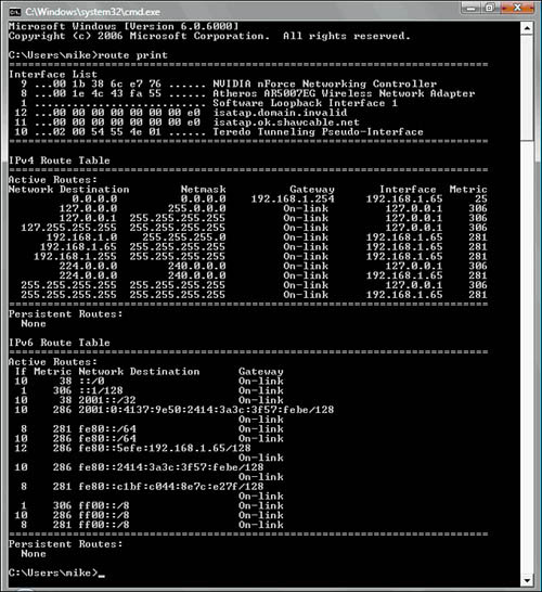
As well as displaying the routing table, the Windows version of the route command has a number of other switches, as detailed in Table 8.13. For complete information about all the switches available with the route command on a Windows system, type route at the command line. To see a list of the route command switches on a Linux system, use the command route --help.

Table 8.13 Switches for the route Command in Windows

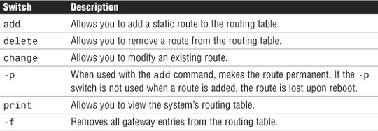
Review and Test Yourself

The following sections provide you with the opportunity to review what you’ve learned in this chapter and to test yourself.

The Facts

For the exam, don’t forget these important concepts:

RAID 0 uses disk striping over two or more disks but offers no fault tolerance.

RAID 1 uses two disks in a mirrored configuration.

Disk duplexing is a RAID 1 implementation using separate hard disk controllers.

RAID 5 is disk striping with parity, requiring three disks at a minimum.

With a full backup, all data is backed up, and data can be restored from a single tape set. Full backups do not use the archive bit but clear it after files have been copied to tape.

With incremental backups, all data that has changed since the last full or incremental backup is backed up. The restore procedure requires several tapes: the latest full backup and all incremental tapes since the last full backup. An incremental backup uses the archive bit and clears it after a file is saved to disk.

With a differential backup, all data changed since the last full backup is backed up. The restore procedure requires the latest full backup tape and the latest differential backup tape. A differential backup uses the archive bit to determine which files need to be backed up but does not clear it.

You should use an offsite tape rotation scheme to store current copies of backups in a secure offsite location. A commonly used rotation is the grandfather, father, son (GFS) rotation.

You should periodically introduce new tapes into the tape rotation and destroy the old ones.

Two key strategies are commonly employed for server fault tolerance: standby servers and server clustering.

Hot, warm, and cold spares are designed to replace failed system components.

Hot, warm, and cold sites are designed to provide alternative locations for network operations in the event of a disaster.

ping is a command-line utility designed to test connectivity between systems on a TCP/IP-based network.

Ping the IP address of your local loopback using the command ping 127.0.0.1. If this command is successful, you know that the TCP/IP protocol suite is installed correctly on your system and is functioning.

If you cannot ping other devices on your local network, but you can ping your local NIC, you might not be connected to the network correctly, or the computer might have a cable problem.

Trace route is a TCP/IP utility that is used to track the path a packet takes to reach a remote host and to isolate where network problems may be. Trace route functionality can be used on Windows platforms with the tracert command and on Linux, UNIX, and Macintosh platforms with the traceroute command.

Trace route reports how long it takes to reach each host in the path. It is a useful tool for isolating bottlenecks in a network.

arp is the part of the TCP/IP suite whose function is to resolve IP addresses to MAC addresses.

arp operates at the network layer of the Open Systems Interconnect (OSI) model.

netstat is used to view both inbound and outbound TCP/IP network connections.

The netstat -r command can be used to display the system’s routing table.

nbtstat is used to display protocol and statistical information for NetBIOS over TCP/IP connections.

The ipconfig command shows the IP configuration information for all NICs installed in a system.

The ipconfig /all command is used to display detailed TCP/IP configuration information.

The ipconfig /renew command is used to renew DHCP assigned IP address configurations.

When looking for client connectivity problems using ipconfig, ensure that the gateway is correctly set.

The ifconfig command is the Linux, Macintosh, and UNIX equivalent of the ipconfig command.

The nslookup command is a TCP/IP diagnostic tool that is used to troubleshoot DNS problems. On Linux, UNIX, and Macintosh systems, you can also use the dig command for the same purpose.

Key Terms

RAID

Disk mirroring

Disk duplexing

Disk striping

Full backup

Incremental backup

Differential backup

Hot site

Cold site

Warm site

Hot spare

Cold spare

tracert

ping

arp

netstat

nbtstat

ipconfig

ifconfig

nslookup

dig

mtr

host

arp ping

route

Exam Prep Questions

1. During your lunch break, you rummage around in the company’s storage closet and discover two 20GB IDE hard disks and two hard disk controllers. You decide to use the equipment to provide a fault-tolerant solution in one of your company’s existing servers. Which of the following fault-tolerant RAID levels could you implement using this equipment? (Choose two.)

A. RAID 0

B. RAID 1

C. Disk duplexing

D. RAID 5

2. Which two types of tape backup methods clear the archive bit after the backup has been completed?

A. Full

B. Differential

C. Incremental

D. GFS

3. You come in to work on Thursday morning to find that the server has failed and you need to restore the data from backup. You finished a full backup on Sunday and incremental backups on Monday, Tuesday, and Wednesday. How many tapes are required to restore the backup?

A. Four

B. Two

C. Three

D. Five

4. In the server room you find a box with five 15GB hard disks. If you were to implement a RAID 5 solution using all five disks, how much storage space would you have for the actual data?

A. 75GB

B. 60GB

C. 30GB

D. 45GB

5. Which of the following RAID levels offers the greatest read and write performance?

A. RAID 0

B. RAID 1

C. Disk duplexing

D. RAID 5

E. RAID 10

6. Which of the following recovery sites might require the delivery of computer equipment and an update of all network data?

A. Cold site

B. Warm site

C. Hot site

D. None of the above

7. As part of your network administrative responsibilities, you have completed your monthly backups. As part of backup best practices, where should the tapes be stored?

A. In a secure location in the server room

B. In a secure location somewhere in the building

C. In an offsite location

D. In a secure offsite location

8. As network administrator, you have been tasked with designing a disaster recovery plan for your network. Which of the following might you include in a disaster recovery plan?

A. RAID 5

B. Offsite tape storage

C. Mirrored hard disks

D. UPS

9. Which of the following power-related problems is associated with a short-term voltage drop?

A. Surge

B. Brownout

C. Sag

D. Spike

10. As a network administrator, you have been asked to implement a RAID solution that offers high performance. Fault tolerance is not a concern. Which RAID level are you likely to use?

A. RAID 0

B. RAID 1

C. RAID 2

D. RAID 5

E. RAID 10

11. Which of the following tools can you use to perform manual DNS lookups on a Linux system? (Choose two.)

A. dig

B. nslookup

C. tracert

D. dnslookup

12. Which of the following commands generates a Request timed out error message?

A. ping

B. netstat

C. ipconfig

D. nbtstat

13. Which of the following commands would you use to add a static entry to the ARP table of a Windows 2000 system?

A. arp -a IP ADDRESS MAC ADDRESS

B. arp -s MAC ADDRESS IP ADDRESS

C. arp -s IP ADDRESS MAC ADDRESS

D. arp -i IP ADDRESS MAC ADDRESS

14. Which command created the following output?

Server: nen.bx.ttfc.net

Address: 209.55.4.155

Name: examcram.com

Address: 63.240.93.157

A. nbtstat

B. ipconfig

C. tracert

D. nslookup

Answers to Exam Prep Questions

1. B, C. Using the equipment you found, you could implement RAID 1, because there are two hard disks for the mirror configuration. You could also implement disk duplexing, because there is an additional hard disk controller. Answer A is incorrect because RAID 0 is not a fault-tolerant RAID level. Answer D is incorrect because RAID 5 requires a minimum of three disks.

2. A, C. The archive bit is reset after a full backup and an incremental backup. Answer B is incorrect because the differential backup does not reset the archive bit. Answer D is wrong because GFS is a rotation strategy, not a backup method.

3. A. Incremental backups save all files and directories that have changed since the last full or incremental backup. To restore, you need the latest full backup and all incremental tapes. In this case, you need four tapes to complete the restore process.

4. B. RAID 5 uses distributed parity. The parity information is spread across all disks and requires the equivalent space of a single hard disk. This example has five 15GB disks, giving a total of 75GB of storage. 15GB is required for the parity information, leaving 60GB for saving actual data.

5. A. Although not a fault-tolerant RAID level, RAID 0 offers the best performance of any RAID level. Other RAID levels do offer some performance improvements over a single disk, but their fault tolerance considerations inhibit the write operations.

6. A. A cold site provides an alternative location but typically not much more. A cold site often requires the delivery of computer equipment and other services. A hot site has all network equipment ready to go in the event of a massive failure. A warm site has most equipment ready but still would need days or weeks to have the network up and running.

7. D. Although not always done, it is a best practice to store tape backups in a secure offsite location in case of fire or theft. Answer A is incorrect because if the server room is damaged by fire or flood, the tapes and the data on the server can be compromised by the same disaster. Similarly, answer B is incorrect because storing the backups onsite does not eliminate the threat of a single disaster destroying the data on the server and tapes. Answer C is incorrect because of security reasons. The offsite tapes must be secured.

8. B. Offsite tape storage is part of a disaster recovery plan. The other answers are considered fault tolerance measures because they are implemented to ensure data availability.

9. C. A sag is a short-term voltage drop. A brownout is also a voltage drop, but it lasts longer than a sag. A surge is an increase in power that lasts a few seconds. A spike is a power increase that lasts a few milliseconds.

10. A. RAID 0 offers the highest level of performance but does not offer any fault tolerance. If the performance of RAID 0 is required and so is fault tolerance, RAID 10 is a better choice. RAID 1 offers fault tolerance but no increase in performance.

11. A, B. Both the dig and nslookup commands can be used to perform manual DNS lookups on a Linux system. You cannot perform a manual lookup with the tracert command. There is no such command as dnslookup.

12. A. The ping command generates a Request timed out error when it is unable to receive a reply from the destination system. None of the other commands listed produce this output.

13. C. This command would correctly add a static entry to the ARP table. None of the other answers are valid ARP switches.

14. D. The output was produced by the nslookup command. The other commands listed produce different output.

Need to Know More?

Mike Harwood. Network+ Prep, 3rd Edition. Que Publishing, 2009.

Douglas Comer. Computer Networks and Internets, 5th Edition. Prentice Hall, 2008.