Chapter 10
Routing Protocols
THE FOLLOWING COMPTIA NETWORK+ EXAM OBJECTIVES ARE COVERED IN THIS CHAPTER:
✓ 1.3 Explain the concepts and characteristics of routing and switching
- Routing
- Routing protocols (IPv4 and IPv6)
- Distance-vector routing protocols
- RIP
- EIGRP
- Link-state routing protocols
- OSPF
- Hybrid
- BGP
- Distance-vector routing protocols
- Routing protocols (IPv4 and IPv6)
- IPv6 concepts
- Tunneling
- Dual stack
- Router advertisement
- Neighbor discovery
✓ 2.2 Given a scenario, determine the appropriate placement of networking devices on a network and install/configure them
- Router
Routing protocols are critical to a network’s design. This chapter focuses on dynamic routing protocols. Dynamic routing protocols run only on routers that use them in order to discover networks and update their routing tables. Using dynamic routing is easier on you, the system administrator, than using the labor-intensive, manually achieved static routing method, but it’ll cost you in terms of router CPU processes and bandwidth on the network links.
The source of the increased bandwidth usage and CPU cycles is the operation of the dynamic routing protocol itself. A router running a dynamic routing protocol shares routing information with its neighboring routers, and it requires additional CPU cycles and additional bandwidth to accomplish that.
In this chapter, I’ll give you all the basic information you need to know about routing protocols so you can choose the correct one for each network you work on or design.
 |
To find Todd Lammle CompTIA videos and practice questions, please see www.lammle.com/network+. |
Routing Protocol Basics
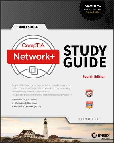
Because getting a solid visual can really help people learn, I’ll get you started by combining the last few figures used in Chapter 9, “Introduction to IP Routing.” This way, you can get the big picture and really understand how routing works. Figure 10.1 shows the complete routing tree that I broke up piece by piece at the end of Chapter 9.
Figure 10.1 Routing flow tree
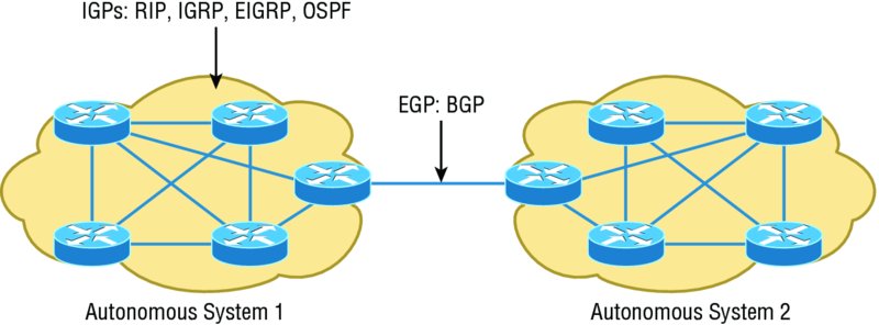
As I touched on in Chapter 9, two types of routing protocols are used in internetworks: interior gateway protocols (IGPs) and exterior gateway protocols (EGPs). IGPs are used to exchange routing information with routers in the same autonomous system (AS). An AS is a collection of networks under a common administrative domain, which simply means that all routers sharing the same routing table information are in the same AS. EGPs are used to communicate between multiple ASs. A nice example of an EGP would be Border Gateway Protocol (BGP).
There are a few key points about routing protocols that I think it would be a good idea to talk over before getting deeper into the specifics of each one. First on the list is something known as an administrative distance.
Administrative Distances
The administrative distance (AD) is used to rate the trustworthiness of routing information received on one router from its neighboring router. An AD is represented as an integer from 0 to 255, where 0 equals the most trusted route and 255 the least. A value of 255 essentially means, “No traffic is allowed to be passed via this route.”
If a router receives two updates listing the same remote network, the first thing the router checks is the AD. If one of the advertised routes has a lower AD than the other, the route with the lower AD is the one that will get placed in the routing table.
If both advertised routes to the same network have the same AD, then routing protocol metrics like hop count or the amount of bandwidth on the lines will be used to find the best path to the remote network. And as it was with the AD, the advertised route with the lowest metric will be placed in the routing table. But if both advertised routes have the same AD as well as the same metrics, then the routing protocol will load-balance to the remote network. To perform load balancing, a router will send packets down each link to test for the best one.
 Real World Scenario
Why Not Just Turn On All Routing Protocols?
Many customers have hired me because all their employees were complaining about a slow, intermittent network that had a lot of latency. Many times, I have found that the administrators did not truly understand routing protocols and just enabled them all on every router.
This may sound laughable, but it is true. When an administrator tried to disable a routing protocol, such as the Routing Information Protocol (RIP), they would receive a call that part of the network was not working. First, understand that because of default ADs, although every routing protocol was enabled, only the Enhanced Interior Gateway Routing Protocol (EIGRP) would show up in most of the routing tables. This meant that Open Shortest Path First (OSPF), Intermediate System-to-Intermediate System (IS-IS), and RIP would be running in the background but just using up bandwidth and CPU processes, slowing the routers almost to a crawl.
Disabling all the routing protocols except EIGRP (this would only work on an all-Cisco router network) improved the network at least 30 percent. In addition, finding the routers that were configured only for RIP and enabling EIGRP solved the calls from users complaining that the network was down when RIP was disabled on the network. Last, I replaced the core routers with better routers with more memory, enabling faster, more efficient routing and raising the network response time to a total of 50 percent.
Table 10.1 shows the default ADs that a router uses to decide which route to take to a remote network.
Table 10.1 Default administrative distances
| Route Source | Default AD |
| Connected interface | 0 |
| Static route | 1 |
| External BGP | 20 |
| Internal EIGRP | 90 |
| IGRP | 100 |
| OSPF | 110 |
| IS-IS | 115 |
| RIP | 120 |
| External EIGRP | 170 |
| Internal BGP | 200 |
| Unknown | 255 (this route will never be used) |
Understand that if a network is directly connected, the router will always use the interface connected to that network. Also good to know is that if you configure a static route, the router will believe that route to be the preferred one over any other routes it learns about dynamically. You can change the ADs of static routes, but by default, they have an AD of 1. That’s only one place above zero, so you can see why a static route’s default AD will always be considered the best by the router.
This means that if you have a static route, a RIP-advertised route, and an EIGRP-advertised route listing the same network, then by default, the router will always use the static route unless you change the AD of the static route.
Classes of Routing Protocols
The three classes of routing protocols introduced in Chapter 9, and shown in Figure 10.1, are as follows:
Distance Vector The distance vector protocols find the best path to a remote network by judging—you guessed it—distance. Each time a packet goes through a router, it equals something we call a hop, and the route with the fewest hops to the destination network will be chosen as the best path to it. The vector indicates the direction to the remote network. RIP, RIPv2, and Interior Gateway Routing Protocol (IGRP) are distance vector routing protocols. These protocols send the entire routing table to all directly connected neighbors.
Link State Using link state protocols, also called shortest path first protocols, the routers each create three separate tables. One of these tables keeps track of directly attached neighbors, one determines the topology of the entire internetwork, and one is used as the actual routing table. Link state routers know more about the internetwork than any distance vector routing protocol. OSPF and IS-IS are IP routing protocols that are completely link state. Link state protocols send updates containing the state of their own links to all other routers on the network.
Hybrid A hybrid protocol uses aspects of both distance vector and link state, and formerly, EIGRP was the only one you needed to understand to meet the Network+ objectives. But now, BGP is also listed as a hybrid routing protocol because of its capability to work as an EGP and be used in supersized internetworks internally. When deployed in this way, it’s called internal BGP, or iBGP, but understand that it’s still most commonly utilized as an EGP.
I also want you to understand that there’s no one set way of configuring routing protocols for use in every situation because this really needs to be done on a case-by-case basis. Even though all of this might seem a little intimidating, if you understand how each of the different routing protocols works, I promise you’ll be capable of making good, solid decisions that will truly meet the individual needs of any business!
Distance Vector Routing Protocols
Okay, the distance vector routing algorithm passes its complete routing table contents to neighboring routers, which then combine the received routing table entries with their own routing tables to complete and update their individual routing tables. This is called routing by rumor because a router receiving an update from a neighbor router believes the information about remote networks without verifying for itself if the news is actually correct.
It’s possible to have a network that has multiple links to the same remote network, and if that’s the case, the AD of each received update is checked first. As I said, if the AD is the same, the protocol will then have to use other metrics to determine the best path to use to get to that remote network.
Distance vector uses only hop count to determine the best path to a network. If a router finds more than one link with the same hop count to the same remote network, it will automatically perform what’s known as round-robin load balancing.
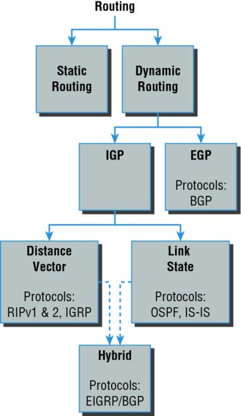
It’s important to understand what a distance vector routing protocol does when it starts up. In Figure 10.2, the four routers start off with only their directly connected networks in their routing table. After a distance vector routing protocol is started on each router, the routing tables are then updated with all route information gathered from neighbor routers.
Figure 10.2 The internetwork with distance vector routing
As you can see in Figure 10.2, each router only has the directly connected networks in its routing table. Also notice that their hop count is zero in every case. Each router sends its complete routing table, which includes the network number, exit interface, and hop count to the network, out to each active interface.
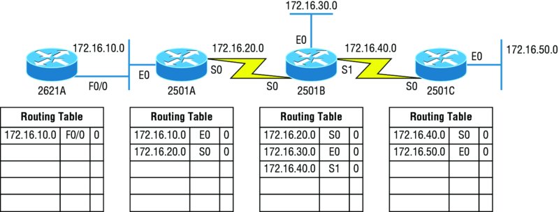
Now, in Figure 10.3, the routing tables are complete because they include information about all the networks in the internetwork. They are considered converged. The hop count for every directly connected network remains zero, but notice that the hop count is incremented by one each time the path completely passes through a router. So, for router 2621A, the path to the 172.16.10.0 network still has a hop count of zero, but the hop count for the path to network 172.16.20.0 is one. The hop count to networks 172.16.30.0 and 172.16.40.0 increases to two, and so on. Usually, data transmission will cease while routers are converging—a good reason in favor of fast convergence time! In fact, one of the main problems with RIP is its slow convergence time.
Figure 10.3 Converged routing tables
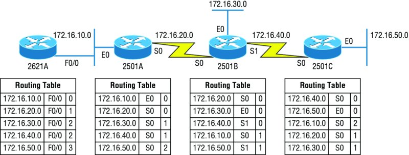
As you can see in Figure 10.3, once all the routers have converged, the routing table in each router keeps information about three important things:
- The remote network number
- The interface that the router will use to send packets to reach that particular network
- The hop count, or metric, to the network
|
Remember! Routing convergence time is the time required by protocols to update their forwarding tables after changes have occurred. |
Let’s start discussing dynamic routing protocols with one of the oldest routing protocols that is still in existence today.
Routing Information Protocol (RIP)
RIP is a true distance vector routing protocol. It sends the complete routing table out to all active interfaces every 30 seconds. RIP uses only one thing to determine the best way to a remote network—the hop count. And because it has a maximum allowable hop count of 15 by default, a hop count of 16 would be deemed unreachable. This means that although RIP works fairly well in small networks, it’s pretty inefficient on large networks with slow WAN links or on networks populated with a large number of routers. Worse, this dinosaur of a protocol has a bad history of creating routing loops, which were somewhat kept in check by using things like maximum hop count. This is the reason why RIP only permits going through 15 routers before it will judge that route to be invalid. If all that isn’t nasty enough for you, RIP also happens to be glacially slow at converging, which can easily cause latency in your network!
RIP version 1 uses only classful routing, which means that all devices in the network must use the same subnet mask for each specific address class. This is because RIP version 1 doesn’t send updates with subnet mask information in tow. RIP version 2 provides something called prefix routing and does send subnet mask information with the route updates. Doing this is called classless routing.
RIP Version 2 (RIPv2)
Let’s spend a couple of minutes discussing RIPv2 before we move into the advanced distance vector (also referred to as hybrid), Cisco-proprietary routing protocol EIGRP.
RIP version 2 is mostly the same as RIP version 1. Both RIPv1 and RIPv2 are distance vector protocols, which means that each router running RIP sends its complete routing tables out to all active interfaces at periodic time intervals. Also, the timers and loop-avoidance schemes are the same in both RIP versions. Both RIPv1 and RIPv2 are configured with classful addressing (but RIPv2 is considered classless because subnet information is sent with each route update), and both have the same AD (120).
But there are some important differences that make RIPv2 more scalable than RIPv1. And I’ve got to add a word of advice here before we move on: I’m definitely not advocating using RIP of either version in your network. But because RIP is an open standard, you can use RIP with any brand of router. You can also use OSPF because OSPF is an open standard as well.
Table 10.2 discusses the differences between RIPv1 and RIPv2.
Table 10.2 RIPv1 vs RIPv2
| RIPv1 | RIPv2 |
| Distance vector | Distance vector |
| Maximum hop count of 15 | Maximum hop count of 15 |
| Classful | Classless |
| Broadcast based | Uses multicast 224.0.0.9 |
| No support for VLSM | Supports VLSM networks |
| No authentication | Allows for MD5 authentication |
| No support for discontiguous networks | Supports discontiguous networks (covered in the next section, “VLSM and Discontiguous Networks”) |
RIPv2, unlike RIPv1, is a classless routing protocol (even though it is configured as classful, like RIPv1), which means that it sends subnet mask information along with the route updates. By sending the subnet mask information with the updates, RIPv2 can support variable length subnet masks (VLSMs), which are described in the next section; in addition, network boundaries are summarized.
VLSM and Discontiguous Networks
VLSMs allow classless routing, meaning that the routing protocol sends subnet-mask information with the route updates. The reason it’s good to do this is to save address space. If we didn’t use a routing protocol that supports VLSMs, then every router interface, every node (PC, printer, server, and so on), would have to use the same subnet mask.
As the name suggests, with VLSMs we can have different subnet masks for different router interfaces. Check out Figure 10.4 to see an example of why classful network designs are inefficient.
Figure 10.4 Typical classful network
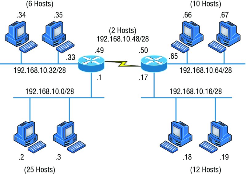
Looking at this figure, you’ll notice that we have two routers, each with two LANs and connected together with a WAN serial link. In a typical classful network design example (RIP or RIPv2 routing protocol), you could subnet a network like this:
- 192.168.10.0 = Network
- 255.255.255.240 (/28) = Mask
Our subnets would be (you know this part, right?) 0, 16, 32, 48, 64, 80, and so on. This allows us to assign 16 subnets to our internetwork. But how many hosts would be available on each network? Well, as you probably know by now, each subnet provides only 14 hosts. This means that with a /28 mask, each LAN can support 14 valid hosts—one LAN requires 25 addresses, so a /28 mask doesn’t provide enough addresses for the hosts in that LAN! Moreover, the point-to-point WAN link also would consume 14 addresses when only 2 are required. It’s too bad we can’t just nick some valid hosts from that WAN link and give them to our LANs.
All hosts and router interfaces have the same subnet mask—again, this is called classful routing. And if we want this network to be more efficient, we definitely need to add different masks to each router interface.
But there’s still another problem—the link between the two routers will never use more than two valid hosts! This wastes valuable IP address space, and it’s the big reason I’m talking to you about VLSM networking.
Now let’s take Figure 10.4 and use a classless design, which will become the new network shown in Figure 10.5. In the previous example, we wasted address space—one LAN didn’t have enough addresses because every router interface and host used the same subnet mask. Not so good.
Figure 10.5 Classless network design
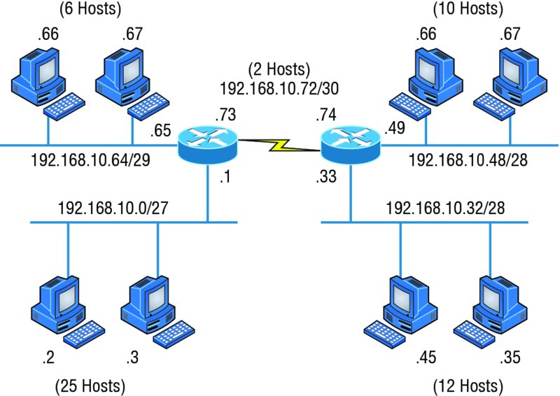
What would be good is to provide only the needed number of hosts on each router interface, meaning VLSMs. Remember that if a “classful routed network” requires that all subnet masks be the same length, then it follows that a “classless routed network” would allow us to use variable length subnet masks (VLSMs).
So, if we use a /30 on our WAN links and a /27, /28, and /29 on our LANs, we’ll get 2 hosts per WAN interface and 30, 14, and 6 hosts per LAN interface—nice! This makes a huge difference—not only can we get just the right number of hosts on each LAN, we still have room to add more WANs and LANs using this same network.
Remember, in order to implement a VLSM design on your network, you need to have a routing protocol that sends subnet-mask information with the route updates. This would be RIPv2, EIGRP, or OSPF. RIPv1 and IGRP will not work in classless networks and are considered classful routing protocols.
|
By using a VLSM design, you do not necessarily make your network run better, but you can save a lot of IP addresses. |
Now, what’s a discontiguous network? It’s one that has two or more subnetworks of a classful network connected together by different classful networks. Figure 10.6 displays a typical discontiguous network.
Figure 10.6 A discontiguous network
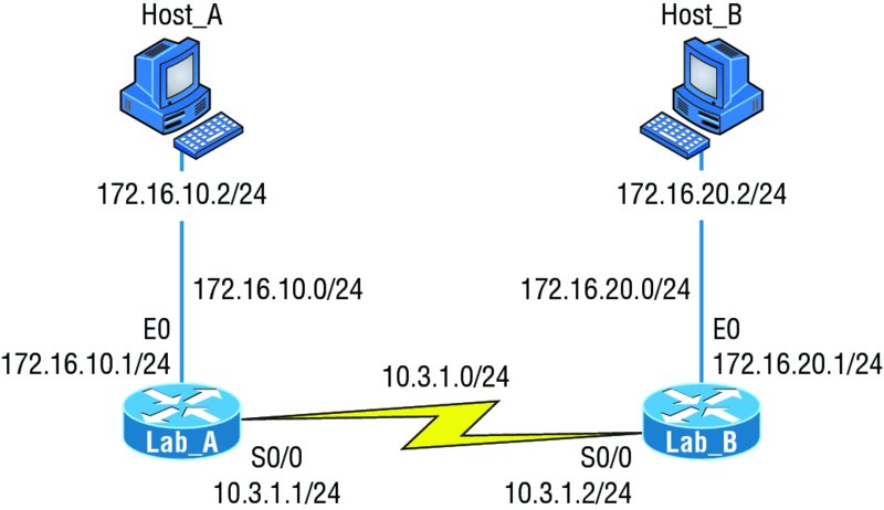
The subnets 172.16.10.0 and 172.16.20.0 are connected together with a 10.3.1.0 network. By default, each router thinks it has the only 172.16.0.0 classful network.
It’s important to understand that discontiguous networks just won’t work with RIPv1 at all. They don’t work by default on RIPv2 or EIGRP either, but discontiguous networks do work on OSPF networks by default because OSPF does not auto-summarize like RIPv2 and EIGRP.
|
Route aggregation is essentially combining multiple subnets into one larger subnet, and it’s also known as supernetting. You would implement this type of route summarization if you required more efficient routing tables in large networks. |
EIGRP
EIGRP is a classless, enhanced distance vector protocol that possesses a real edge over another older Cisco proprietary protocol, IGRP. That’s basically why it’s called Enhanced IGRP.
EIGRP uses the concept of an autonomous system to describe the set of contiguous routers that run the same routing protocol and share routing information. But unlike IGRP, EIGRP includes the subnet mask in its route updates. And as you now know, the advertisement of subnet information allows us to use VLSMs when designing our networks.
EIGRP is referred to as a hybrid routing protocol because it has characteristics of both distance vector and link state protocols. For example, EIGRP doesn’t send link state packets as OSPF does; instead, it sends traditional distance vector updates containing information about networks, plus the cost of reaching them from the perspective of the advertising router. But EIGRP has link state characteristics as well—it synchronizes routing tables between neighbors at startup and then sends specific updates only when topology changes occur. This makes EIGRP suitable for very large networks.
There are a number of powerful features that make EIGRP a real standout from RIP, RIPv2, and other protocols. The main ones are listed here:
- Support for IP and IPv6 (and some other useless routed protocols) via protocol-dependent modules
- Considered classless (same as RIPv2 and OSPF)
- Support for VLSM/Classless Inter-Domain Routing (CIDR)
- Support for summaries and discontiguous networks
- Efficient neighbor discovery
- Communication via Reliable Transport Protocol (RTP)
- Best path selection via Diffusing Update Algorithm (DUAL)
Another great feature of EIGRP is that it’s simple to configure and turn on like a distance vector protocol, but it keeps track of more information than a distance vector does. It creates and maintains additional tables instead of just one table as distance vector routing protocols do. To determine the best path to each network, EIGRP uses bandwidth and delay of the line as well as sending reliability, load, and the MTU information between routers, but it only uses bandwidth and delay by default.
These tables are called the neighbor table, topology table, and routing table, as shown in Figure 10.7.
Figure 10.7 EIGRP tables
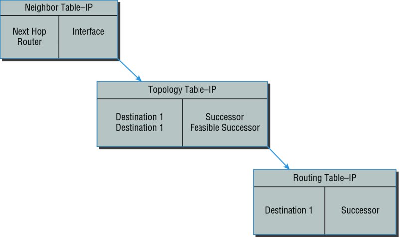
Neighbor Table Each router keeps state information about adjacent neighbors. When a newly discovered neighbor is learned on a router interface, the address and interface of that neighbor are recorded, and the information is held in the neighbor table and stored in RAM. Sequence numbers are used to match acknowledgments with update packets. The last sequence number received from the neighbor is recorded so that out-of-order packets can be detected.
Topology Table The topology table is populated by the neighbor table, and the best path to each remote network is found by running Diffusing Update Algorithm (DUAL). The topology table contains all destinations advertised by neighboring routers, holding each destination address and a list of neighbors that have advertised the destination. For each neighbor, the advertised metric, which comes only from the neighbor’s routing table, is recorded. If the neighbor is advertising this destination, it must be using the route to forward packets.
Successor (Routes in a Routing Table) A successor route (think successful!) is the best route to a remote network. A successor route is used by EIGRP to forward traffic to a destination and is stored in the routing table. It is backed up by a feasible successor route that is stored in the topology table—if one is available.
Feasible Successor (Backup Routes) A feasible successor is a path considered a backup route. EIGRP will keep up to six feasible successors in the topology table. Only the one with the best metric (the successor) is copied and placed in the routing table.
By using the feasible distance and having feasible successors in the topology table as backup links, EIGRP allows the network to converge instantly and updates to any neighbor only consist of traffic sent from EIGRP. All of these things make for a very fast, scalable, fault-tolerant routing protocol.
|
Route redistribution is the term used for translating from one routing protocol into another. An example would be where you have an old router running RIP but you have an EIGRP network. You can run route redistribution on one router to translate the RIP routes into EIGRP. |
Border Gateway Protocol (BGP)
In a way, you can think of Border Gateway Protocol (BGP) as the heavyweight of routing protocols. This is an external routing protocol (used between autonomous systems, unlike RIP or OSPF, which are internal routing protocols) that uses a sophisticated algorithm to determine the best route.
|
Even though BGP is an EGP by default, it can be used within an AS, which is one of the reasons the objectives are calling this a hybrid routing protocol. Another reason they call it a hybrid is because it’s often known as a path vector protocol instead of a distance vector like RIP. |
In fact, it just happens to be the core routing protocol of the Internet. And it’s not exactly breaking news that the Internet has become a vital resource in so many organizations, is it? No—but this growing dependence has resulted in redundant connections to many different ISPs.
This is where BGP comes in. The sheer onslaught of multiple connections would totally overwhelm other routing protocols like OSPF, which I am going to talk about shortly. BGP is essentially an alternative to using default routes for controlling path selections. Default routes are configured on routers to control packets that have a destination IP address that is not found in the routing table. Please see CCNA Routing and Switching Complete Study Guide: Exam 100-105, Exam 200-105, Exam 200-125, 2nd Edition for more information on static and default routing.
Because the Internet’s growth rate shows no signs of slowing, ISPs use BGP for its ability to make classless routing and summarization possible. These capabilities help to keep routing tables smaller and more efficient at the ISP core.
BGP is used for IGPs to connect ASs together in larger networks, if needed, as shown in Figure 10.8.
Figure 10.8 Border Gateway Protocol (BGP)
|
An autonomous system is a collection of networks under a common administrative domain. IGPs operate within an autonomous system, and EGPs connect different autonomous systems together. |
So yes, very large private IP networks can make use of BGP. Let’s say you wanted to join a number of large OSPF networks together. Because OSPF just couldn’t scale up enough to handle such a huge load, you would go with BGP instead to connect the ASs together. Another situation in which BGP would come in really handy would be if you wanted to multi-home a network for better redundancy, either to a multiple access point of a single ISP or to multiple ISPs.
Internal routing protocols are employed to advertise all available networks, including the metric necessary to get to each of them. BGP is a personal favorite of mine because its routers exchange path vectors that give you detailed information on the BGP AS numbers, hop by hop (called an AS path), required to reach a specific destination network. Also good to know is that BGP doesn’t broadcast its entire routing table like RIP does; it updates a lot more like OSPF, which is a huge advantage. Also, the routing table with BGP is called a Routing Information Base (RIB).
And BGP also tells you about any/all networks reachable at the end of the path. These factors are the biggest differences you need to remember about BGP. Unlike IGPs that simply tell you how to get to a specific network, BGP gives you the big picture on exactly what’s involved in getting to an AS, including the networks located in that AS itself.
And there’s more to that “BGP big picture”—this protocol carries information like the network prefixes found in the AS and includes the IP address needed to get to the next AS (the next-hop attribute). It even gives you the history on how the networks at the end of the path were introduced into BGP in the first place, known as the origin code attribute.
All of these traits are what makes BGP so useful for constructing a graph of loop-free autonomous systems, for identifying routing policies, and for enabling us to create and enforce restrictions on routing behavior based upon the AS path—sweet!
Link State Routing Protocols
Link state protocols also fall into the classless category of routing protocols, and they work within packet-switched networks. OSPF and IS-IS are two examples of link state routing protocols.
Remember, for a protocol to be a classless routing protocol, the subnet-mask information must be carried with the routing update. This enables every router to identify the best route to each and every network, even those that don’t use class-defined default subnet masks (i.e., 8, 16, or 24 bits), such as VLSM networks. All neighbor routers know the cost of the network route that’s being advertised. One of the biggest differences between link state and distance vector protocols is that link state protocols learn and maintain much more information about the internetwork than distance vector routing protocols do. Distance vector routing protocols only maintain routing tables with the destination routes and vector costs (like hop counts) in them. Link state routing protocols maintain two additional tables with more detailed information, with the first of these being the neighbor table. The neighbor table is maintained through the use of hello packets that are exchanged by all routers to determine which other routers are available to exchange routing data with. All routers that can share routing data are stored in the neighbor table.
The second table maintained is the topology table, which is built and sustained through the use of link state advertisements or packets (LSAs or LSPs). In the topology table, you’ll find a listing for every destination network plus every neighbor (route) through which it can be reached. Essentially, it’s a map of the entire internetwork.
Once all of that raw data is shared and each one of the routers has the data in its topology table, the routing protocol runs the Shortest Path First (SPF) algorithm to compare it all and determine the best paths to each of the destination networks.
Open Shortest Path First (OSPF)
Open Shortest Path First (OSPF) is an open-standard routing protocol that’s been implemented by a wide variety of network vendors, including Cisco. OSPF works by using the Dijkstra algorithm. First, a shortest-path tree is constructed, and then the routing table is populated with the resulting best paths. OSPF converges quickly (although not as fast as EIGRP), and it supports multiple, equal-cost routes to the same destination. Like EIGRP, it supports both IP and IPv6 routed protocols, but OSPF must maintain a separate database and routing table for each, meaning you’re basically running two routing protocols if you are using IP and IPv6 with OSPF.
OSPF provides the following features:
- Consists of areas and autonomous systems
- Minimizes routing update traffic
- Allows scalability
- Supports VLSM/CIDR
- Has unlimited hop count
- Allows multivendor deployment (open standard)
- Uses a loopback (logical) interface to keep the network stable
OSPF is the first link state routing protocol that most people are introduced to, so it’s good to see how it compares to more traditional distance vector protocols like RIPv2 and RIPv1. Table 10.3 gives you a comparison of these three protocols.
Table 10.3 OSPF and RIP comparison
| Characteristic | OSPF | RIPv2 | RIPv1 |
| Type of protocol | Link state | Distance vector | Distance vector |
| Classless support | Yes | Yes | No |
| VLSM support | Yes | Yes | No |
| Auto-summarization | No | Yes | Yes |
| Manual summarization | Yes | No | No |
| Discontiguous support | Yes | Yes | No |
| Route propagation | Multicast on change | Periodic multicast | Periodic broadcast |
| Path metric | Bandwidth | Hops | Hops |
| Hop-count limit | None | 15 | 15 |
| Convergence | Fast | Slow | Slow |
| Peer authentication | Yes | Yes | No |
| Hierarchical network | Yes (using areas) | No (flat only) | No (flat only) |
| Updates | Event triggered | Route table updates time intervals | Route table updates |
| Route computation | Dijkstra | Bellman-Ford | Bellman-Ford |
OSPF has many features beyond the few I’ve listed in Table 10.3, and all of them contribute to a fast, scalable, and robust protocol that can be actively deployed in thousands of production networks. One of OSPF’s most noteworthy features is that after a network change, such as when a link changes to up or down, OSPF converges with serious speed! In fact, it’s the fastest of any of the interior routing protocols we’ll be covering. Just to make sure you’re clear, convergence refers to when all routers have been successfully updated with the change.
OSPF is supposed to be designed in a hierarchical fashion, which basically means that you can separate the larger internetwork into smaller internetworks called areas. This is definitely the best design for OSPF.
The following are reasons you really want to create OSPF in a hierarchical design:
- To decrease routing overhead
- To speed up convergence
- To confine network instability to single areas of the network
Pretty sweet benefits! But you have to earn them—OSPF is more elaborate and difficult to configure in this manner.
Figure 10.9 shows a typical OSPF simple design. Notice how each router connects to the backbone—called area 0, or the backbone area. OSPF must have an area 0, and all other areas should connect to this area. Routers that connect other areas to the backbone area within an AS are called area border routers (ABRs). Still, at least one interface of the ABR must be in area 0.
Figure 10.9 OSPF design example
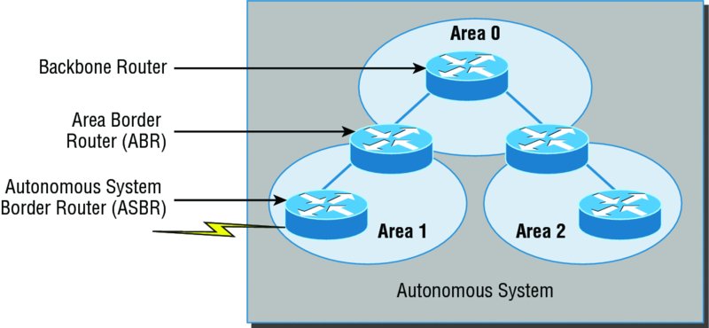
OSPF runs inside an autonomous system, but it can also connect multiple autonomous systems together. The router that connects these ASs is called an autonomous system border router (ASBR). Typically, in today’s networks, BGP is used to connect between ASs, not OSPF.
Ideally, you would create other areas of networks to help keep route updates to a minimum and to keep problems from propagating throughout the network. But that’s beyond the scope of this chapter. Just make note of it for your future networking studies.
Intermediate System-to-Intermediate System (IS-IS)
IS-IS is an IGP, meaning that it’s intended for use within an administrative domain or network, not for routing between ASs. That would be a job that an EGP (such as BGP, which we just covered) would handle instead.
IS-IS is a link state routing protocol, meaning it operates by reliably flooding topology information throughout a network of routers. Each router then independently builds a picture of the network’s topology, just as they do with OSPF. Packets or datagrams are forwarded based on the best topological path through the network to the destination.
Figure 10.10 shows an IS-IS network and the terminology used with IS-IS.
Figure 10.10 IS-IS network terminology
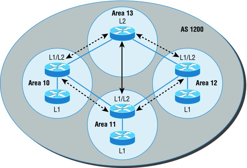
Here are the definitions for the terms used in the IS-IS network shown in Figure 10.10 :
L1 Level 1 intermediate systems route within an area. When the destination is outside an area, they route toward a Level 2 system.
L2 Level 2 intermediate systems route between areas and toward other ASs.
The similarity between IS-IS and OSPF is that both employ the Dijkstra algorithm to discover the shortest path through the network to a destination network. The difference between IS-IS and OSPF is that IS-IS uses Connectionless Network Service (CLNS) to provide connectionless delivery of data packets between routers, and it also doesn’t require an area 0 like OSPF does. OSPF uses IP to communicate between routers instead.
An advantage to having CLNS around is that it can easily send information about multiple routed protocols (IP and IPv6), and as I already mentioned, OSPF must maintain a completely different routing database for IP and IPv6, respectively, for it to be able to send updates for both protocols.
IS-IS supports the most important characteristics of OSPF and EIGRP because it supports VLSM and also because it converges quickly. Each of these three protocols has advantages and disadvantages, but it’s these two shared features that make any of them scalable and appropriate for supporting the large-scale networks of today.
One last thing—even though it’s not as common, IS-IS, although comparable to OSPF, is actually preferred by ISPs because of its ability to run IP and IPv6 without creating a separate database for each protocol as OSPF does. That single feature makes it more efficient in very large networks.
High Availability
First hop redundancy protocols (FHRPs) work by giving you a way to configure more than one physical router to appear as if they were only a single logical one. This makes client configuration and communication easier because you can simply configure a single default gateway and the host machine can use its standard protocols to communicate. First hop is a reference to the default router being the first router, or first router hop, through which a packet must pass.
So how does a redundancy protocol accomplish this? The protocols I’m going to describe to you do this basically by presenting a virtual router to all of the clients. The virtual router has its own IP and MAC addresses. The virtual IP address is the address that’s configured on each of the host machines as the default gateway. The virtual MAC address is the address that will be returned when an ARP request is sent by a host. The hosts don’t know or care which physical router is actually forwarding the traffic, as you can see in Figure 10.11.
Figure 10.11 FHRPs use a virtual router with a virtual IP address and virtual MAC address.
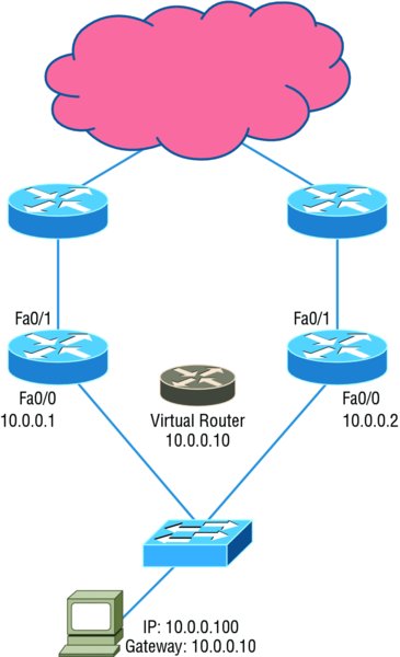
It’s the responsibility of the redundancy protocol to decide which physical router will actively forward traffic and which one will be placed in standby in case the active router fails. Even if the active router fails, the transition to the standby router will be transparent to the hosts because the virtual router, identified by the virtual IP and MAC addresses, is now used by the standby router. The hosts never change default gateway information, so traffic keeps flowing.
|
Fault-tolerant solutions provide continued operation in the event of a device failure, and load-balancing solutions distribute the workload over multiple devices. |
Next we’ll explore these two important redundancy protocols:
Hot Standby Router Protocol (HSRP) This is by far Cisco’s favorite protocol ever! Don’t buy just one router; buy up to eight routers to provide the same service, and keep seven as backup in case of failure! HSRP is a Cisco proprietary protocol that provides a redundant gateway for hosts on a local subnet, but this isn’t a load-balanced solution. HSRP allows you to configure two or more routers into a standby group that shares an IP address and MAC address and provides a default gateway. When the IP and MAC addresses are independent from the routers’ physical addresses (on a virtual interface, not tied to a specific interface), they can swap control of an address if the current forwarding and active router fails. But there is actually a way you can sort of achieve load balancing with HSRP—by using multiple VLANs and designating a specific router for one VLAN, then an alternate router as active for VLAN via trunking.
Virtual Router Redundancy Protocol (VRRP) This also provides a redundant—but again, not load-balanced—gateway for hosts on a local subnet. It’s an open standard protocol that functions almost identically to HSRP. I’ll comb through the fine differences that exist between these protocols.
Hot Standby Router Protocol (HSRP)
Again, HSRP is a Cisco proprietary protocol that can be run on most, but not all, of Cisco’s router and multilayer switch models. It defines a standby group, and each standby group that you define includes the following routers:
- Active router
- Standby router
- Virtual router
- Any other routers that may be attached to the subnet
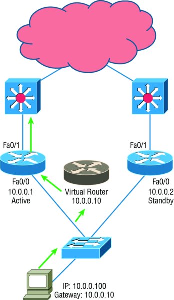
The problem with HSRP is that with it, only one router is active and two or more routers just sit there in standby mode and won’t be used unless a failure occurs—not very cost effective or efficient! Figure 10.12 shows how only one router is used at a time in an HSRP group.
Figure 10.12 HSRP active and standby routers
The standby group will always have at least two routers participating in it. The primary players in the group are the one active router and one standby router that communicate to each other using multicast Hello messages. The Hello messages provide all of the required communication for the routers. The Hellos contain the information required to accomplish the election that determines the active and standby router positions. They also hold the key to the failover process. If the standby router stops receiving hello packets from the active router, it then takes over the active router role, as shown in Figure 10.13.
Figure 10.13 Example of HSRP active and standby routers swapping interfaces
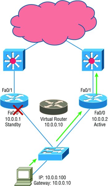
As soon as the active router stops responding to Hellos, the standby router automatically becomes the active router and starts responding to host requests.
Virtual MAC Address
A virtual router in an HSRP group has a virtual IP address and a virtual MAC address. So where does that virtual MAC come from? The virtual IP address isn’t that hard to figure out; it just has to be a unique IP address on the same subnet as the hosts defined in the configuration. But MAC addresses are a little different, right? Or are they? The answer is yes—sort of. With HSRP, you create a totally new, made-up MAC address in addition to the IP address.
The HSRP MAC address has only one variable piece in it. The first 24 bits still identify the vendor who manufactured the device (the organizationally unique identifier, or OUI). The next 16 bits in the address tells us that the MAC address is a well-known HSRP MAC address. Finally, the last 8 bits of the address are the hexadecimal representation of the HSRP group number.
Let me clarify all this with an example of what an HSRP MAC address would look like:
0000.0c07.ac0a
- The first 24 bits (0000.0c) are the vendor ID of the address; in the case of HSRP being a Cisco protocol, the ID is assigned to Cisco.
- The next 16 bits (07.ac) are the well-known HSRP ID. This part of the address was assigned by Cisco in the protocol, so it’s always easy to recognize that this address is for use with HSRP.
- The last 8 bits (0a) are the only variable bits and represent the HSRP group number that you assign. In this case, the group number is 10 and converted to hexadecimal when placed in the MAC address, where it becomes the 0a that you see.
You can see this MAC address added to the ARP cache of every router in the HSRP group. There will be the translation from the IP address to the MAC address as well as the interface on which it’s located.
HSRP Timers
Before we get deeper into the roles that each of the routers can have in an HSRP group, I want to define the HSRP timers. The timers are very important to HSRP function because they ensure communication between the routers, and if something goes wrong, they allow the standby router to take over. The HSRP timers include hello, hold, active, and standby.
Hello Timer The hello timer is the defined interval during which each of the routers send out Hello messages. Their default interval is 3 seconds, and they identify the state that each router is in. This is important because the particular state determines the specific role of each router and, as a result, the actions each will take within the group. Figure 10.14 shows the Hello messages being sent, and the router uses the hello timer to keep network traffic flowing in case of a failure.
Figure 10.14 HSRP Hellos
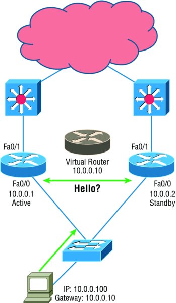
This timer can be changed, and people used to avoid doing so because it was thought that lowering the hello value would place an unnecessary load on the routers. That isn’t true with most of the routers today; in fact, you can configure the timers in milliseconds, meaning the failover time can be in milliseconds! Still, keep in mind that increasing the value will make the standby router wait longer before taking over for the active router when it fails or can’t communicate.
Hold Timer The hold timer specifies the interval the standby router uses to determine whether the active router is offline or out of communication. By default, the hold timer is 10 seconds, roughly three times the default for the hello timer. If one timer is changed for some reason, I recommend using this multiplier to adjust the other timers too. By setting the hold timer at three times the hello timer, you ensure that the standby router doesn’t take over the active role every time there’s a short break in communication.
Active Timer The active timer monitors the state of the active router. The timer resets each time a router in the standby group receives a hello packet from the active router. This timer expires based on the hold time value that’s set in the corresponding field of the HSRP Hello message.
Standby Timer The standby timer is used to monitor the state of the standby router. The timer resets anytime a router in the standby group receives a hello packet from the standby router and expires based on the hold time value that’s set in the respective hello packet.
Real World Scenario
Large Enterprise Network Outages with FHRPs
Years ago when HSRP was all the rage, and before VRRP, enterprises used hundreds of HSRP groups. With the hello timer set to 3 seconds and a hold time of 10 seconds, these timers worked just fine and we had great redundancy with our core routers.
However, as we’ve seen in the last few years, and will certainly see in the future, 10 seconds is now a lifetime! Some of my customers have been complaining with the failover time and loss of connectivity to their virtual server farms.
So lately I’ve been changing the timers to well below the defaults. Cisco had changed the timers so you could use sub-second times for failover. Because these are multicast packets, the overhead that is seen on a current high-speed network is almost nothing.
The hello timer is typically set to 200 msec and the hold time is 700 msec. The command is as follows:
(config-if)#Standby 1 timers msec 200 msec 700
This almost ensures that not even a single packet is lost when there is an outage.
Virtual Router Redundancy Protocol
Like HSRP, Virtual Router Redundancy Protocol (VRRP) allows a group of routers to form a single virtual router. In an HSRP or VRRP group, one router is elected to handle all requests sent to the virtual IP address. With HSRP, this is the active router. An HSRP group has only one active router, at least one standby router, and many listening routers. A VRRP group has one master router and one or more backup routers and is the open standard implementation of HSRP.
Comparing VRRP and HSRP
The LAN workstations are configured with the address of the virtual router as their default gateway, just as they are with HSRP, but VRRP differs from HSRP in these important ways:
- VRRP is an IEEE standard (RFC 2338) for router redundancy; HSRP is a Cisco proprietary protocol.
- The virtual router that represents a group of routers is known as a VRRP group.
- The active router is referred to as the master virtual router.
- The master virtual router may have the same IP address as the virtual router group.
- Multiple routers can function as backup routers.
- VRRP is supported on Ethernet, Fast Ethernet, and Gigabit Ethernet interfaces as well as on Multiprotocol Label Switching (MPLS), virtual private networks (VPNs), and VLANs.
VRRP Redundancy Characteristics
VRRP has some unique features:
- VRRP provides redundancy for the real IP address of a router or for a virtual IP address shared among the VRRP group members.
- If a real IP address is used, the router with that address becomes the master.
- If a virtual IP address is used, the master is the router with the highest priority.
- A VRRP group has one master router and one or more backup routers.
- The master router uses VRRP messages to inform group members of its status.
- VRRP allows load sharing across more than one virtual router.
Advanced IPv6 Concepts
Before we jump into the coverage of IPv6 routing protocols, we need to discuss some of the operations that are performed differently in IPv6 than in IPv4 and that includes several operations that are radically different. We’ll also discuss in the following sections some of the methods that have been developed over the past few years to ease the pain of transitioning to an IPv6 environment from one that is IPv4.
Router Advertisement
A router advertisement is part of a new system configuration option in IPv6. This a packet sent by routers to give the host a network ID ( called a prefix in IPv6) so that the host can generate its own IPv6 address derived from its MAC address.
To perform auto-configuration, a host goes through a basic three-step process:
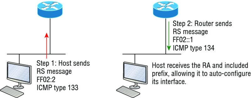
- First, the host needs the prefix information, similar to the network portion of an IPv4 address, to configure its interface, so it sends a router solicitation (RS) request for it. This RS is then sent out as a multicast to all routers (FF02::2). The actual information being sent is a type of ICMP message, and like everything in networking, this ICMP message has a number that identifies it. The RS message is ICMP type 133.
- The router answers back with the required prefix information via a router advertisement (RA). An RA message also happens to be a multicast packet that’s sent to the all-nodes multicast address (FF02::1) and is ICMP type 134. RA messages are sent on a periodic basis, but the host sends the RS for an immediate response so it doesn’t have to wait until the next scheduled RA to get what it needs.
- Upon receipt, the host will generate an IPv6 address. The exact process used (stateless or stateful auto-configuration or by DHCPv6) is determined by instructions within the RA.
The first two steps are shown in Figure 10.15.
Figure 10.15 First two steps to IPv6 auto-configuration
By the way, when the host generates an IPV6 address using the prefix and its MAC address the process is called stateless auto-configuration because it doesn’t contact or connect to and receive any further information from the other device.
Take a look at Figure 10.16. In this figure, the Branch router needs to be configured, but I just don’t feel like typing in an IPv6 address on the interface connecting to the Corp router. I also don’t feel like typing in any routing commands, but I need more than a link-local address on that interface, so I’m going to have to do something! So basically, I want to have the Branch router work with IPv6 on the internetwork with the least amount of effort from me. Let’s see if I can get away with that.
Figure 10.16 IPv6 auto-configuration example
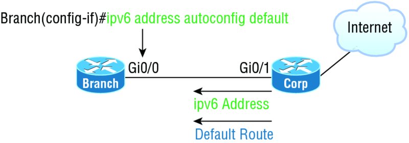
Aha—there is an easy way! I love IPv6 because it allows me to be relatively lazy when dealing with some parts of my network, yet it still works really well. When I use the command ipv6 address autoconfig, the interface will listen for RAs and then, via the EUI-64 format, it will assign itself a global address—sweet!
Neighbor Discovery
One of the big changes in IPv6 is the discontinuation of the use of all broadcasts, including the ARP broadcast. Devices use a new process to send to one another within a subnet. They send to one another’s link-local address rather than the MAC addresses. Even devices that have been assigned an IPv6 address manually will still generate a link-local address. These addresses are generated using the MAC address as is done in stateless auto-configuration; the prefix is not learned from the router. A link-local address always adopts a prefix of FE80::/64.
That means that rather than needing to learn a MAC address to send locally, the host needs to learn the link-local addresses of all of the other hosts in its subnet. This is done using a process called neighbor discovery. This is done using neighbor solicitation messages and neighbor advertisement messages. These are both sent to IPv6 multicast addresses that have been standardized for this process.
Neighbor solicitation messages are sent on the local link when a host needs the link-layer address of another node (see Figure 10.17). The source address in a neighbor solicitation message is the IPv6 address of the node sending the neighbor solicitation message. The destination address in the neighbor solicitation message is the solicited-node multicast address that corresponds to the IPv6 address of the destination node. The neighbor solicitation message also includes the link-layer address of the source node.
Figure 10.17 IPv6 neighbor discovery: neighbor solicitation message
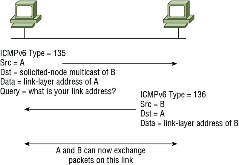
The destination node replies by sending a neighbor advertisement message, which has a value of 136 in the Type field of the ICMP packet header, on the local link. The data portion of the neighbor advertisement message includes the link-layer address of the node sending the neighbor advertisement message. After the source node receives the neighbor advertisement, the source node and destination node can communicate.
Tunneling
When tunneling is used as a transition mechanism to IPv6, it involves encapsulating one type of protocol in another type of protocol for the purpose of transmitting it across a network that supports the packet type or protocol. At the tunnel endpoint, the packet is deencapsulated and the contents are then processed in its native form.
Overlay tunneling encapsulates IPv6 packets in IPv4 packets for delivery across an IPv4 network. Overlay tunnels can be configured between border routers or between a border router and a host capable of supporting both IPv6 and IPv4. Cisco IOS supports the following tunnel types:
- Manual
- Routing encapsulation (GRE)
- 6to4
- ISATAP
Some of the more significant methods are covered in the following sections.
GRE Tunnels
Although not used as an IPv6 transition mechanism, Generic Routing Encapsulation (GRE) tunnels are worth discussing while talking about tunneling. GRE is a general-purpose encapsulation that allows for transporting packets from one network through another network through a VPN. One of its benefits is its ability to use a routing protocol. It also can carry non-IP traffic, and when implemented as a GRE over IPsec tunnel, it supports encryption. When this type of tunnel is built, the GRE encapsulation will occur before the IPSec encryption process. One key thing to keep in mind is that the tunnel interfaces on either end must be in the same subnet.
6to4 Tunneling
6to4 tunneling is super useful for carrying IPv6 data over a network that is still IPv4. In some cases, you will have IPv6 subnets or portions of your network that are all IPv6, and those networks will have to communicate with each other. This could happen over a WAN or some other network that you do not control. So how do we fix this problem? By creating a tunnel that will carry the IPv6 traffic for you across the IPv4 network. Now having a tunnel is not that hard, and it isn’t difficult to understand. It is really taking the IPv6 packet that would normally be traveling across the network, grabbing it up, and placing an IPv4 header on the front of it that specifies an IPv4 protocol type of 41.
When you’re configuring either a manual or automatic tunnel (covered in the next two sections), three key pieces must be configured:
- The tunnel mode
- The IPv4 tunnel source
- A 6to4 IPv6 address that lies within 2002 ::/16
Manual IPv6 Tunneling
In order to make this happen we are going to have a couple of dual-stacked routers. We just have to add a little configuration to place a tunnel between the routers. Tunnels are very simple. We just have to tell each router where the tunnel is starting and where it has to end up. Let’s take a look. The following configuration creates what is known as a manual IPv6 tunnel.
Router1(config)#int tunnel 0
Router1(config-if)#ipv6 address 2001:db8:1:1::1/64
Router1(config-if)#tunnel source 192.168.30.1
Router1(config-if)#tunnel destination 192.168.40.1
Router1(config-if)#tunnel mode ipv6ip
Router2(config)#int tunnel 0
Router2(config-if)#ipv6 address 2001:db8:2:2::1/64
Router2(config-if)#tunnel source 192.168.40.1
Router2(config-if)#tunnel destination 192.168.30.1
Router2(config-if)#tunnel mode ipv6ip
This will allow our IPv6 networks to communicate over the IPv4 network. Now this is not meant to be a permanent configuration. The end goal should be to have an all-IPv6 network end to end.
6to4 (Automatic)
The following configuration uses what is known as automatic 6to4 tunneling. This allows for the endpoints to auto-configure an IPv6 address where a site-specific /48 bit prefix is dynamically constructed by prepending the prefix 2002 to an IPv4 address assigned to the site. This means the first 2 bytes of the IPv6 address will be 0x2002 and the next 4 bytes will be the hexadecimal equivalent of the IPv4 address. Therefore, in this case 192.168.99.1 translates to 2002:c0a8:6301:: /48. Tunnel interface 0 is configured without an IPv4 or IPv6 address because the IPv4 or IPv6 addresses on Ethernet interface 0 are used to construct a tunnel source address. A tunnel destination address is not specified because the destination address is automatically constructed. It is also possible for each tunnel to have multiple destinations, which is not possible when creating a manual IPv6 tunnel.
Router(config)# interface ethernet 0
Router(config-if)# ip address 192.168.99.1 255.255.255.0
Router(config-if)# ipv6 address 2002:c0a8:6301::/48 eui-64
Router(config-if)# exit
Router(config)# interface tunnel 0
Router(config-if)# no ip address
Router(config-if)# ipv6 unnumbered ethernet 0
Router(config-if)# tunnel source ethernet 0
Router(config-if)# tunnel mode ipv6ip 6to4
Router(config-if)# exit
When using automatic 6to4 tunnels, in many cases you will need to reference the tunnel endpoint when creating the neighbor statement (for example, in BGP). When doing so, you can refer to the auto-configured address in the preceding example in three ways in the neighbor command.
:: c0a8:6301
:: 192.168.99.1
0:0:0:0:0:0:192.168.99.1
To configure a static route to a network that needs to cross a 6to4 tunnel, use the ipv6 route command. When you do so, the least significant 32 bits of the address referenced by the command will correspond to the IPv4 address assigned to the tunnel source. For example, in the following command, the final 32 bits will be the IPv4 address of the tunnel 0 interface.
Ipv6 route 2002::/16 tunnel 0
ISATAP Tunneling
Intra-Site Automatic Tunnel Addressing Protocol is another mechanism for transmitting IPv6 packets over an IPv4 network. The word automatic means that once an ISATAP server/router has been set up, only the clients must be configured to connect to it. A sample configuration is shown here.
R1(config)#ipv6 unicast-routing
R1(config)#interface tunnel 1
R1(config-if)# tunnel source ethernet 0
R1(config-if)# tunnel mode ipv6ip isatap
R1(config-if)# ipv6 address 2001:DB8::/64 eui-64
One other thing that maybe noteworthy: if the IPv4 network that you are traversing in this situation has a NAT translation point, it will break the tunnel encapsulation that we have created. In the following section, a solution is discussed.
Teredo
Teredo gives full IPv6 connectivity for IPv6 hosts that are on an IPv4 network but have no direct native connection to an IPv6 network. Its distinguishing feature is that it is able to perform its function even from behind Network Address Translation (NAT) devices such as home routers.
The Teredo protocol performs several functions:
- Diagnoses UDP over IPv4 (UDPv4) connectivity and discovers the kind of NAT present (using a simplified replacement to the STUN protocol)
- Assigns a globally routable unique IPv6 address to each host
- Encapsulates IPv6 packets inside UDPv4 datagrams for transmission over an IPv4 network (this includes NAT traversal)
- Routes traffic between Teredo hosts and native (or otherwise non-Teredo) IPv6 hosts
There are several components that can make up the Teredo infrastructure:
Teredo Client A host that has IPv4 connectivity to the Internet from behind a NAT device and uses the Teredo tunneling protocol to access the IPv6 Internet.
Teredo Server A well-known host that is used for initial configuration of a Teredo.
Teredo Relay The remote end of a Teredo tunnel. A Teredo relay must forward all of the data on behalf of the Teredo clients it serves, with the exception of direct Teredo client to Teredo client exchanges.
Teredo Host-Specific Relay A Teredo relay whose range of service is limited to the very host it runs on.
Dual Stack
This is the most common type of migration strategy. It allows the devices to communicate using either IPv4 or IPv6. This technique allows for one-by-one upgrade of applications and devices on the network. As more and more things on the network are upgraded, more of your communication will occur over IPv6. Eventually all devices and software will be upgraded and the IPv4 protocol stacks can be removed. The configuration of dual stacking on a Cisco router is very easy. It requires nothing more than enabling IPv6 forwarding and applying an address to the interfaces that are already configured with IPv4. It will look something like this.
Corp(config)#ipv6 unicast-routing
Corp(config)#interface fastethernet 0/0
Corp(config-if)#ipv6 address 2001:db8:3c4d:1::/64 eui-64
Corp(config-if)#ip address 192.168.255.1 255.255.255.0
IPv6 Routing Protocols
Most of the routing protocols we’ve already discussed have been upgraded for use in IPv6 networks. Also, many of the functions and configurations that we’ve already learned will be used in almost the same way as they’re used now. Knowing that broadcasts have been eliminated in IPv6, it follows that any protocols that use entirely broadcast traffic will go the way of the dodo—but unlike the dodo, it’ll be good to say good-bye to these bandwidth-hogging, performance-annihilating little gremlins!
The routing protocols that we’ll still use in version 6 got a new name and a facelift. Let’s talk about a few of them now.
First on the list is RIPng (next generation). Those of you who have been in IT for a while know that RIP has worked very well for us on smaller networks, which happens to be the reason it didn’t get whacked and will still be around in IPv6. And we still have EIGRPv6 because it already had protocol-dependent modules and all we had to do was add a new one to it for the IPv6 protocol. Rounding out our group of protocol survivors is OSPFv3—that’s not a typo; it really is version 3. OSPF for IPv4 was actually version 2, so when it got its upgrade to IPv6, it became OSPFv3.
RIPng
To be honest, the primary features of RIPng are the same as they were with RIPv2. It is still a distance vector protocol, has a max hop count of 15, and still has the same loop avoidance mechanisms as well as using UDP port 521.
And it still uses multicast to send its updates, too, but in IPv6, it uses FF02::9 for the transport address. This is actually kind of cool because in RIPv2, the multicast address was 224.0.0.9, so the address still has a 9 at the end in the new IPv6 multicast range. In fact, most routing protocols got to keep a little bit of their IPv4 identities like that.
But of course there are differences in the new version or it wouldn’t be a new version, would it? We know that routers keep the next-hop addresses of their neighbor routers for every destination network in their routing table. The difference is that with RIPng, the router keeps track of this next-hop address using the link-local address, not a global address. So just remember that RIPng will pretty much work the same way as with IPv4.
EIGRPv6
As with RIPng, EIGRPv6 works much the same as its IPv4 predecessor does—most of the features that EIGRP provided before EIGRPv6 will still be available.
EIGRPv6 is still an advanced distance vector protocol that has some link state features. The neighbor-discovery process using Hellos still happens, and it still provides reliable communication with a reliable transport protocol that gives us loop-free fast convergence using DUAL.
Hello packets and updates are sent using multicast transmission, and as with RIPng, EIGRPv6’s multicast address stayed almost the same. In IPv4 it was 224.0.0.10; in IPv6, it’s FF02::A (A = 10 in hexadecimal notation).
Last to check out in our group is what OSPF looks like in the IPv6 routing protocol.
OSPFv3
The new version of OSPF continues the trend of the routing protocols having many similarities with their IPv4 versions.
The foundation of OSPF remains the same—it is still a link state routing protocol that divides an entire internetwork or autonomous system into areas, making a hierarchy.
Adjacencies (neighbor routers running OSPF) and next-hop attributes now use link-local addresses, and OSPFv3 still uses multicast traffic to send its updates and acknowledgments, with the addresses FF02::5 for OSPF routers and FF02::6 for OSPF-designated routers, which provide topological updates (route information) to other routers. These new addresses are the replacements for 224.0.0.5 and 224.0.0.6, respectively, which were used in OSPFv2.
With all this routing information behind you, it’s time to go through some review questions and then move on to learning all about switching in the next chapter.
|
Shortest Path Bridging (SPB), specified in the IEEE 802.1aq standard, is a computer networking technology intended to simplify the creation and configuration of networks and replace the older 802.1d/802.1w protocols while enabling multipath routing |
Summary
This chapter covered the basic routing protocols that you may find on a network today. Probably the most common routing protocols you’ll run into are RIP, OSPF, and EIGRP.
I covered RIP, RIPv2, and the differences between the two RIP protocols as well as EIGRP, and BGP in the section on distance vector protocols. We also covered IPv6 routing protocols and some advanced IPv6 operations, including transitional mechanisms such as dual stacking and tunneling.
I finished by discussing OSPF and IS-IS and when you would possibly see each one in a network.
Exam Essentials
Remember the differences between RIPv1 and RIPv2. RIPv1 sends broadcasts every 30 seconds and has an AD of 120. RIPv2 sends multicasts (224.0.0.9) every 30 seconds and also has an AD of 120. RIPv2 sends subnet mask information with the route updates, which allows it to support classless networks and discontiguous networks. RIPv2 also supports authentication between routers, and RIPv1 does not.
Compare OSPF and RIPv1. OSPF is a link state protocol that supports VLSM and classless routing; RIPv1 is a distance vector protocol that does not support VLSM and supports only classful routing.
Written Lab
You can find the answers to the written labs in Appendix A.
-
The default administrative distance of RIP is .
-
The default administrative distance of EIGRP is .
-
The default administrative distance of RIPv2 is .
-
What is the default administrative distance of a static route?
-
What is the version or name of RIP that is used with IPv6?
-
What is the version or name of OSPF that is used with IPv6?
-
What is the version or name of EIGRP that is used with IPv6?
-
When would you use BGP?
-
When could you use EIGRP?
-
Is BGP considered link state or distance vector routing protocol?
Review Questions
You can find the answers to the review questions in Appendix B.
-
Which of the following protocols support VLSM, summarization, and discontiguous networking? (Choose three.)
- RIPv1
- IGRP
- EIGRP
- OSPF
- BGP
- RIPv2
-
Which of the following are considered distance vector routing protocols? (Choose two.)
- OSPF
- RIP
- RIPv2
- IS-IS
-
Which of the following are considered link state routing protocols? (Choose two.)
- OSPF
- RIP
- RIPv2
- IS-IS
-
Which of the following is considered a hybrid routing protocol? (Choose two.)
- OSPF
- BGP
- RIPv2
- IS-IS
- EIGRP
-
Why would you want to use a dynamic routing protocol instead of using static routes?
- There is less overhead on the router.
- Dynamic routing is more secure.
- Dynamic routing scales to larger networks.
- The network runs faster.
-
Which of the following is a vendor-specific FHRP protocol?
- STP
- OSPF
- RIPv1
- EIGRP
- IS-IS
- HSRP
-
RIP has a long convergence time and users have been complaining of response time when a router goes down and RIP has to reconverge. Which can you implement to improve convergence time on the network?
- Replace RIP with static routes.
- Update RIP to RIPv2.
- Update RIP to OSPF using link state.
- Replace RIP with BGP as an exterior gateway protocol.
-
What is the administrative distance of OSPF?
- 90
- 100
- 110
- 120
-
Which of the following protocols will advertise routed IPv6 networks?
- RIP
- RIPng
- OSPFv2
- EIGRPv3
-
What is the difference between static and dynamic routing?
- You use static routing in large, scalable networks.
- Dynamic routing is used by a DNS server.
- Dynamic routes are added automatically.
- Static routes are added automatically.
-
Which routing protocol has a maximum hop count of 15?
- RIPv1
- IGRP
- EIGRP
- OSPF
-
Which of the following describes routing convergence time?
- The time it takes for your VPN to connect
- The time required by protocols to update their forwarding tables after changes have occurred
- The time required for IDS to detect an attack
- The time required by switches to update their link status and go into forwarding state
-
What routing protocol is typically used to connect ASs on the Internet?
- IGRP
- RIPv2
- BGP
- OSPF
-
RIPv2 sends out its routing table every 30 seconds just like RIPv1, but it does so more efficiently. What type of transmission does RIPv2 use to accomplish this task?
- Broadcasts
- Multicasts
- Telecast
- None of the above
-
Which routing protocols have an administrative distance of 120? (Choose two.)
- RIPv1
- RIPv2
- EIGRP
- OSPF
-
Which of the following routing protocols uses AS-Path as one of the methods to build the routing tables?
- OSPF
- IS-IS
- BGP
- RIP
- EIGRP
-
Which IPv6 routing protocol uses UDP port 521?
- RIPng
- EIGRPv6
- OSPFv3
- IS-IS
-
What EIGRP information is held in RAM and maintained through the usage of hello and update packets? (Select all that apply.)
- DUAL table
- Neighbor table
- Topology table
- Successor route
-
Which is true regarding EIGRP successor routes?
- Successor routes are saved in the neighbor table.
- Successor routes are stored in the DUAL table.
- Successor routes are used only if the primary route fails.
- A successor route is used by EIGRP to forward traffic to a destination.
-
Which of the following uses only hop count as a metric to find the best path to a remote network?
- RIP
- EIGRP
- OSPF
- BGP