
The mind is not a vessel to be filled, but a fire to be kindled.—Plutarch
We humans are blessed with extraordinary powers of mind. These powers allow us to differentiate and distinguish, develop new skills, learn new arts, and make rational decisions. Our visual powers have no limits. We can recognize faces regardless of pose and background. We can distinguish objects like cars, dogs, tables, phones, and so on irrespective of the brand and type. We can recognize colors and shapes and distinguish clearly and easily between them. This power is developed periodically and systematically. In our young age, we continuously learn the attributes of objects and develop our knowledge. That information is kept safe in our memory. With time, this knowledge and learning improve. This is such an astonishing process that iteratively trains our eyes and minds. It is often argued that Deep Learning originated as a mechanism to mimic these extraordinary powers. In computer vision, Deep Learning is helping us to uncover the capabilities which can be used to help organizations use computer vision for productive purposes. Deep Learning has evolved a lot and is still having a lot of scope for further progress.
In the first chapter, we started with fundamentals of Deep Learning. In this second chapter, we will build on those fundamentals, go deeper, understand the various layers of a Neural Network, and create a Deep Learning solution using Keras and Python.
- (1)
What is tensor and how to use TensorFlow
- (2)
Demystifying Convolutional Neural Network
- (3)
Components of convolutional Neural Network
- (4)
Developing CNN network for image classification
2.1 Technical requirements
The code and datasets for the chapter are uploaded at the GitHub link https://github.com/Apress/computer-vision-using-deep-learning/tree/main/Chapter2 for this book. We will use the Jupyter Notebook. For this chapter, a CPU is good enough to execute the code, but if required you can use Google Colaboratory. You can refer to the reference at the end of the book, if you are not able to set up the Google Colab yourself.
2.2 Deep Learning using TensorFlow and Keras
Let us examine TensorFlow (TF) and Keras briefly now. They are arguably the most common open source libraries.
TensorFlow (TF) is a platform for Machine Learning by Google. Keras is a framework developed on top of other DL toolkits like TF, Theano, CNTK, and so on. It has built-in support for convolutional and recurrent Neural Networks.
Keras is an API-driven solution; most of the heavy lifting is already done in Keras. It is easier to use and hence recommended for beginners.
The computations in TF are done using data flow graphs wherein the data is represented by edges (which are nothing but tensors or multidimensional data arrays) and nodes that represent mathematical operations. So, what exactly are tensors?
2.3 What is a tensor?
Recall scalars and vectors from your high-school mathematics. Vectors can be visualized as scalars with a direction. For example, a speed of 50 km/hr is a scalar, while 50 km/hr in the north direction is a vector. This means that a vector is a scalar magnitude in a given direction. A tensor, on the other hand, will be in multiple directions, that is, scalar magnitudes in multiple directions.
In terms of a mathematical definition, a tensor is an object that can provide a linear mapping between two algebraic objects. These objects can themselves be scalars or vectors or even tensors.
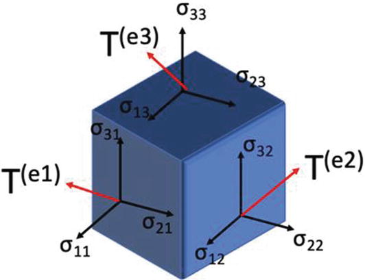
A tensor represented in a vector space diagram. A tensor is a scalar magnitude in multiple directions and is used to provide linear mapping between two algebraic objects
As you can see in Figure 2-1, a tensor has projections across multiple directions. A tensor can be thought of as a mathematical entity, which is described using components. They are described with reference to a basis, and if this associated basis changes, the tensor has to change itself. An example is coordinate change; if a transformation is done on the basis, the tensor’s numeric value will also change. TensorFlow uses these tensors to make complex computations.
Now let’s develop a basic check to see if you have installed TF correctly. We are going to multiply two constants to check if the installation is correct.
Refer to Chapter 1 if you want to know how to install TensorFlow and Keras.
- 1.
Let’s import TensorFlow:
- 2.
Initialize two constants:
- 3.
Multiply the two constants:
- 4.
Print the final result:
If you are able to get the results, congratulations you are all set to go!
Now let us study a Convolutional Neural Network in detail. After that, you will be ready to create your first image classification model.
Exciting, right?
2.3.1 What is a Convolutional Neural Network?
When we humans see an image or a face, we are able to identify it immediately. It is one of the basic skills we have. This identification process is an amalgamation of a large number of small processes and coordination between various vital components of our visual system.
A Convolutional Neural Network or CNN is able to replicate this astounding capability using Deep Learning.
Consider this. We have to create a solution to distinguish between a cat and a dog. The attributes which make them different can be ears, whiskers, nose, and so on. CNNs are helpful for extracting the attributes of the images which are significant for the images. Or in other words, CNNs will extract the features which are distinguishing between a cat and a dog. CNNs are very powerful in image classification, object detection, object tracking, image captioning, face recognition, and so on.
Let us dive into the concepts of CNN. We will examine convolution first.
2.3.2 What is convolution?
The primary objective of the convolution process is to extract features which are important for image classification, object detection, and so on. The features will be edges, curves, color drops, lines and so on. Once the process has been trained well, it will learn these attributes at a significant point in the image. And then it can detect it later in any part of the image.

Convolution process: input layer is on the left, output is on the right. The 32x32 image is being convoluted by a filter of size 5x5
The 5x5 area which is passed over the entire image is called a filter which is sometimes called a kernel or feature detector. The region which is highlighted in Figure 2-2 is called the filter’s receptive field. Hence, we can say that a filter is just a matrix with values called weights. These weights are trained and updated during the model training process. This filter moves over each and every part of the image.

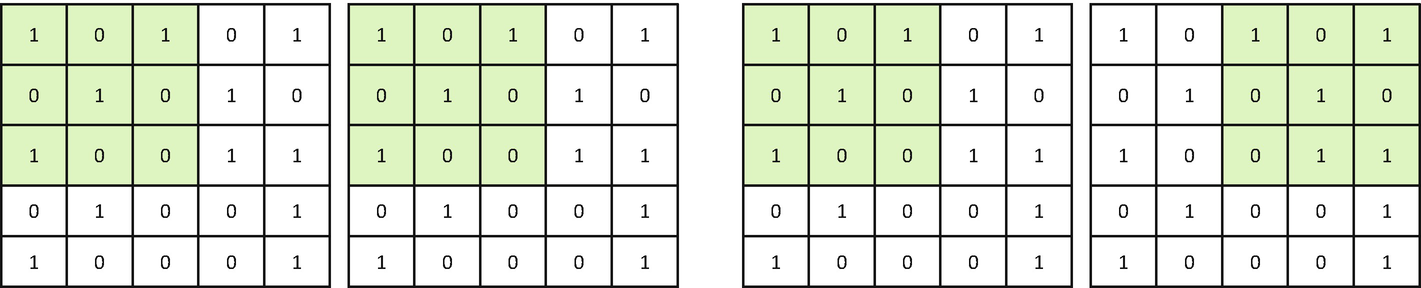
Convolution is the process where the element-wise product and the addition are done. In the first image, the output is 3, and in the second image, the filter has shifted one place to the right and the output is 2
In Figure 2-3, the 3x3 filter is convolving over the entire image. The filter checks if the feature it meant to detect is present or not. The filter carries a convolution process, which is the element-wise product and sum between the two metrics. If a feature is present, the convolution output of the filter and the part of the image will result in a high number. If the feature is not present, the output will be low. Hence, this output value represents how confident a filter is that a particular feature is present in the image.
We move this filter over the entire image, resulting in an output matrix called feature maps or activation maps. This feature map will have the convolutions of the filter over the entire image.
Let’s say the dimensions of the input image are (n,n) and the dimensions of filter are (x,x).
So, the output after the CNN layer is ((n-x+1), (n-x+1)).
Hence, in the example in Figure 2-3, the output is (5-3+1, 5-3+1) = (3,3).
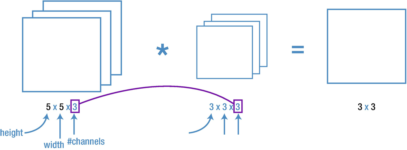
The filter has the same number of channels as the input image
Stride suggests how much the filter should move at each step. The figure shows the impact of a stride on convolution. In the first figure, we have a stride of 1, while in the second image, we have a stride of 2
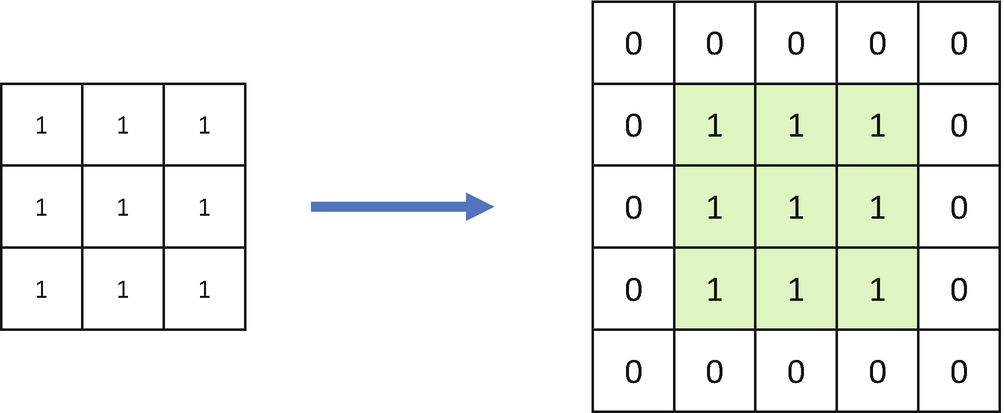
Zero padding has been added to the input image. Convolution as the process reduces the number of pixels, padding allows us to tackle it
Now we have understood the prime components of a CNN. Let us combine the concepts and create a small process. If we have an image of size (nxn) and we apply a filter of size “f,” with a stride of “s” and padding “s,” then the output of the process will be
((n+2p – f)/s +1), (n+2p – f)/s +1)) (Equation 2-1)
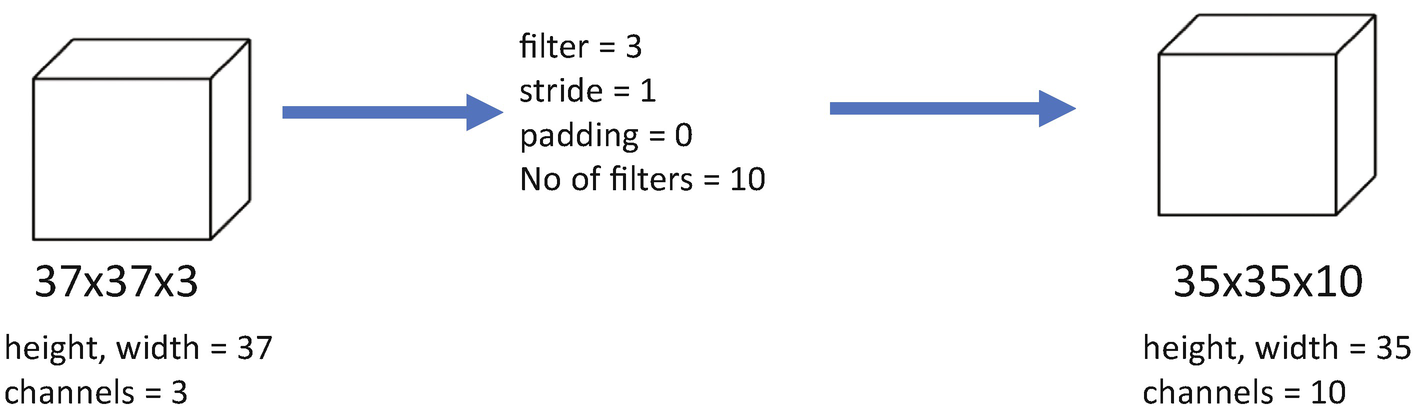
A convolution process in which we have a filter of size 3x3, stride of 1, padding of 0, and number of filters as 10
Convolution helps us in extracting the significant attributes of the image. The layers of the network closer to the origin (the input image) learn the low-level features, while the final layers learn the higher features. In the initial layers of the network, features like edges, curves, and so on are getting extracted, while the deeper layers will learn about the resulting shapes from these low-level features like face, object, and so on.
But this computation looks complex, isn’t it? And as the network will go deep, this complexity will increase. So how do we deal with it? Pooling layer is the answer. Let’s understand it.
2.3.3 What is a Pooling Layer?
The CNN layer which we studied results in a feature map of the input. But as the network becomes deeper, this computation becomes complex. It is due to the reason that with each layer and neuron, the number of dimensions in the network increases. And hence the overall complexity of the network increases.
And, there’s one more challenge: any image augmentation will change the feature map. For example, a rotation will change the position of a feature in the image, and hence the respective feature map will also change.
Often, you will face nonavailability of raw data. Image augmentation is one of the recommended methods to create new images for you which can serve as training data.
This change in the feature map can be addressed by downsampling. In downsampling, a lower resolution of the input image is created, and the Pooling Layer helps us with this.
A Pooling Layer is added after the Convolutional Layer. Each of the feature maps is operated upon individually, and we get a new set of pooled feature maps. The size of this operation filter is smaller than the feature map’s size.
A pooling layer is generally applied after the convolutional layer. A pooling layer with 3x3 pixels and a stride diminishes feature maps’ size by a factor of 2 which means that each dimension is halved. For example, if we apply a pooling layer to a feature map of 8x8 (64 pixels), the output will be a feature map of 4x4 (16 pixels).
There are two types of Pooling Layers.

The right figure is the max pooling, while the bottom is the average pooling
As you can see in Figure 2-8, the average pooling layer does an average of the four numbers, while the max pooling selects the maximum from the four numbers.
There is one more important concept about Fully Connected layers which you should know before you are equipped to create a CNN model. Let us examine it and then you are good to go.
2.3.4 What is a Fully Connected Layer?
A Fully Connected layer takes input from the outputs of the preceding layer (activation maps of high-level features) and outputs an n-dimensional vector. Here, n is the number of distinct classes.
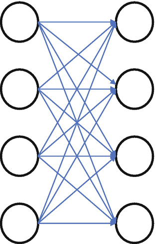
A fully connected layer is depicted here
A Fully Connected layer will look at the features which correspond most closely to a particular class and have particular weights. This is done to get correct probabilities for different classes when we get the product between the weights and the previous layer.
Now you have understood CNN and its components. It is time to hit the code. You will create your first Deep Learning solution to classify between cats and dogs. All the very best!
2.4 Developing a DL solution using CNN
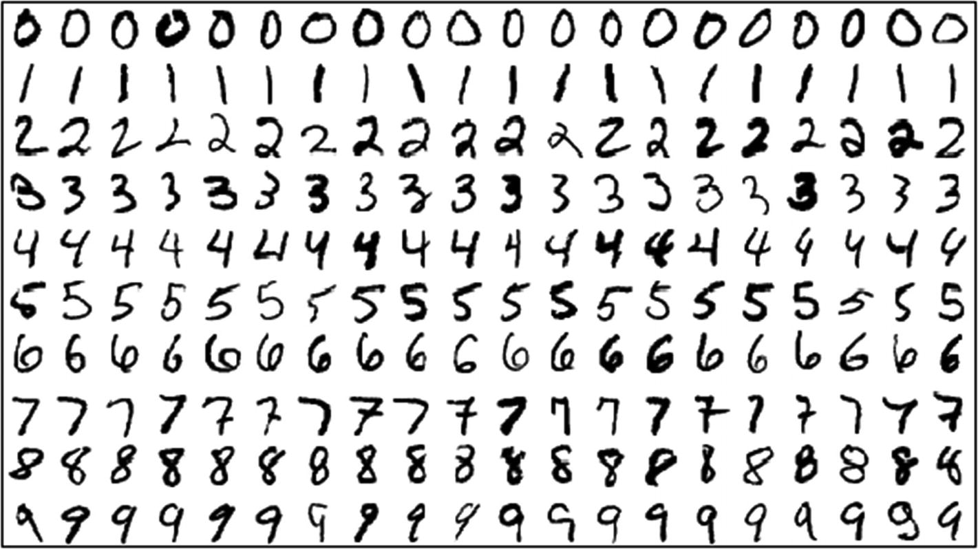
MNIST dataset: “Hello World” for image recognition
There is a famous paper on recognizing MNIST images (description is given at the end of the chapter). To avoid repetition, we are uploading the entire code at GitHub. You are advised to check the code.
We will now start creating the image classification model!
In this first Deep Learning solution, we want to distinguish between a cat and a dog based on their image. The dataset is available at www.kaggle.com/c/dogs-vs-cats.
- 1.First, let’s build the dataset:
- a.
Download the dataset from Kaggle. Unzip the dataset.
- b.
You will find two folders: test and train. Delete the test folder as we will create our own test folder.
- c.
Inside both the train and test folders, create two subfolders – cats and dogs – and put the images in the respective folders.
- d.
Take some images (I took 2000) from the “train>cats” folder and put them in the “test>cats” folder.
- e.
Take some images (I took 2000) from the “train>dogs” folder and put them in the “test>dogs” folder.
- f.
Your dataset is ready to be used.
- 2.
Import the required libraries now. We will import sequential, pooling, activation, and flatten layers from keras. Import numpy too.
Note In the Reference of the book, we provide the description of each of the layers and their respective functions.
from keras.models import Sequentialfrom keras.layers import Conv2D,Activation,MaxPooling2D,Dense,Flatten,Dropoutimport numpy as np - 3.
Initialize a model, catDogImageclassifier variable here:
catDogImageclassifier = Sequential() - 4.Now, we’ll add layers to our network. Conv2D will add a two-dimensional convolutional layer which will have 32 filters. 3,3 represents the size of the filter (3 rows, 3 columns). The following input image shape is 64*64*3 – height*width*RGB. Each number represents the pixel intensity (0–255).catDogImageclassifier.add(Conv2D(32,(3,3),input_shape=(64,64,3)))
- 5.
The output of the last layer will be a feature map. The training data will work on it and get some feature maps.
- 6.
Let’s add the activation function. We are using ReLU (Rectified Linear Unit) for this example. In the feature map output from the previous layer, the activation function will replace all the negative pixels with zero.
Note Recall from the definition of ReLU; it is max(0,x). ReLU allows positive values while replaces negative values with 0. Generally, ReLU is used only in hidden layers.
- 7.Now we add the Max Pooling layer as we do not want our network to be overly complex computationally.catDogImageclassifier.add(MaxPooling2D(pool_size =(2,2)))
- 8.Next, we add all three convolutional blocks. Each block has a Cov2D, ReLU, and Max Pooling Layer.catDogImageclassifier.add(Conv2D(32,(3,3))) catDogImageclassifier.add(Activation('relu')) catDogImageclassifier.add(MaxPooling2D(pool_size =(2,2))) catDogImageclassifier.add(Conv2D(32,(3,3))) catDogImageclassifier.add(Activation('relu')) catDogImageclassifier.add(MaxPooling2D(pool_size =(2,2))) catDogImageclassifier.add(Conv2D(32,(3,3 catDogImageclassifier.add(Activation('relu')) catDogImageclassifier.add(MaxPooling2D(pool_size =(2,2)))
- 9.
Now, let’s flatten the dataset which will transform the pooled feature map matrix into one column.
catDogImageclassifier.add(Flatten()) - 10.Add the dense function now followed by the ReLU activation:catDogImageclassifier.add(Dense(64)) catDogImageclassifier.add(Activation('relu'))
Info Do you think why we need nonlinear functions like tanh, ReLU, and so on? If you use only linear functions, the output will be linear too. Hence, we use nonlinear functions in hidden layers.
- 11.
Overfitting is a nuisance. We will add the Dropout layer to overcome overfitting next:
catDogImageclassifier.add(Dropout(0.5)) - 12.
Add one more fully connected layer to get the output in n-dimensional classes (a vector will be the output).
catDogImageclassifier.add(Dense(1)) - 13.
Add the Sigmoid function to convert to probabilities:
catDogImageclassifier.add(Activation('sigmoid')) - 14.
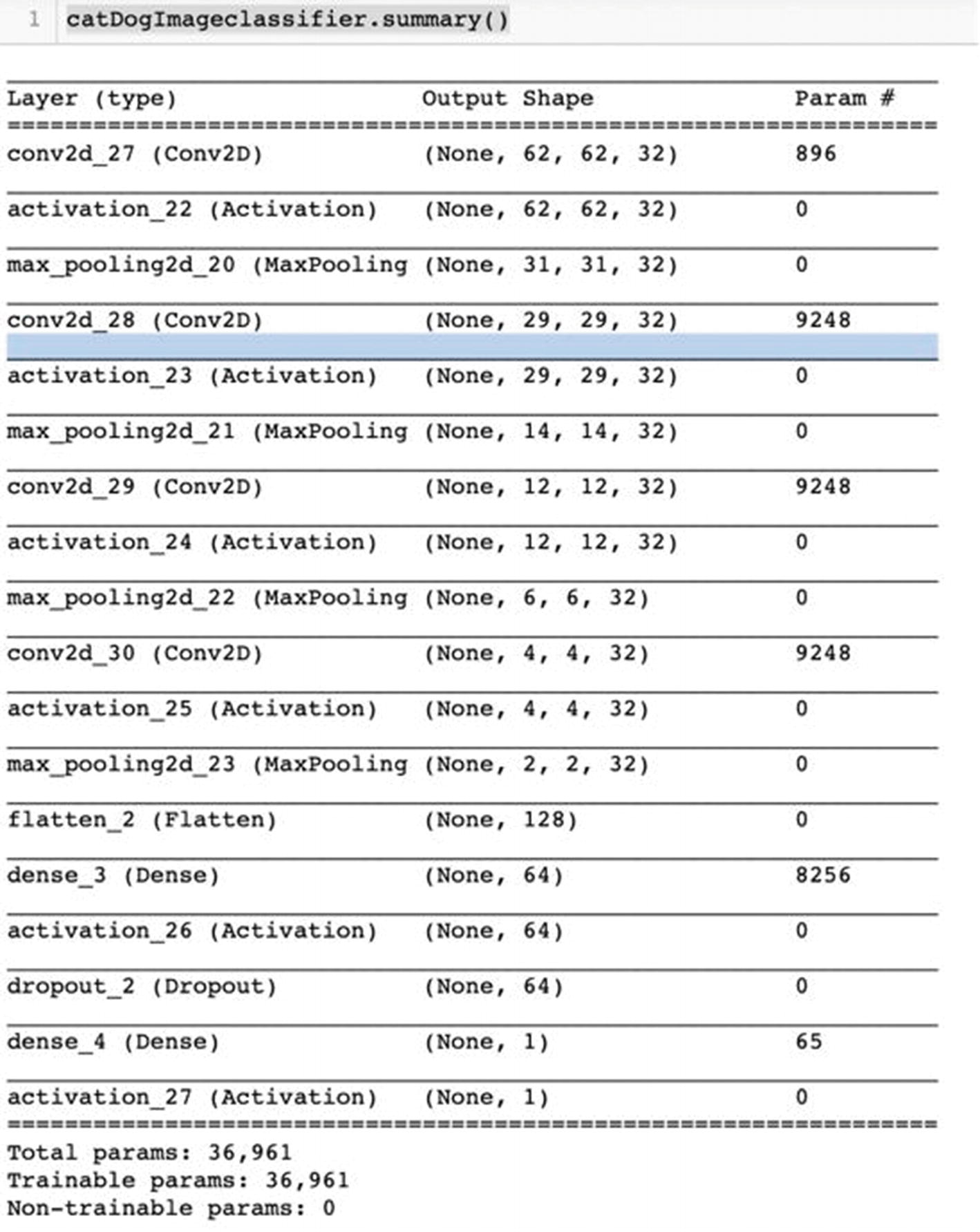
Let’s print a summary of the network.
catDogImageclassifier.summary()
We see the entire network in the following image:
- 15.Let us now compile the network. We use the optimizer rmsprop using gradient descent, and then we add the loss or the cost function.catDogImageclassifier.compile(optimizer ='rmsprop', loss ='binary_crossentropy',metrics =['accuracy'])
- 16.Now we are doing data augmentation here (zoom, scale, etc.). It will also help to tackle the problem of overfitting. We use the ImageDataGenerator function to do this:from keras.preprocessing.image import ImageDataGeneratortrain_datagen = ImageDataGenerator(rescale =1./255, shear_range =0.25,zoom_range = 0.25, horizontal_flip =True)test_datagen = ImageDataGenerator(rescale = 1./255)
- 17.Load the training data:training_set = train_datagen.flow_from_directory('/Users/DogsCats/train',target_size=(64,6 4),batch_size= 32,class_mode='binary')
- 18.Load the testing data:test_set = test_datagen.flow_from_directory('/Users/DogsCats/test', target_size = (64,64),batch_size = 32,class_mode ='binary')
- 19.Let us begin the training now.from IPython.display import displayfrom PIL import Image catDogImageclassifier.fit_generator(training_set, steps_per_epoch =625,epochs = 10, validation_data =test_set, validation_steps = 1000)
Steps per epoch are 625, and the number of epochs is 10. If we have 1000 images and a batch size of 10, the number of steps required will be 100 (1000/10).
The number of epochs means the number of complete passes through the full training dataset. Batch is the number of training examples in a batch, while iteration is the number of batches needed to complete an epoch.
Depending on the complexity of the network, the number of epochs given, and so on, the compilation will take time. The test dataset is passed as a validation_data here.
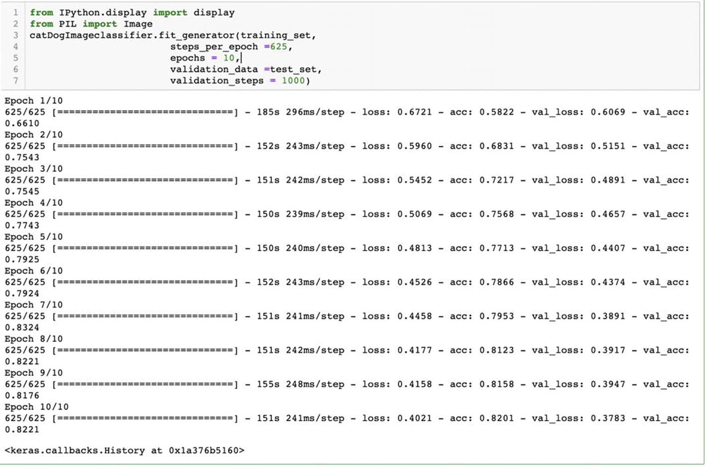
Output of the training results for 10 epochs
As seen in the results, in the final epoch, we got validation accuracy of 82.21%. We can also see that in Epoch 7 we got an accuracy of 83.24% which is better than the final accuracy.
We would then want to use the model created in Epoch 7 as the accuracy is best for it. We can achieve it by providing checkpoints between the training and saving that version. We will look at the process of creating and saving checkpoints in subsequent chapters.
- 20.Load the saved model using load_model:from keras.models import load_modelcatDogImageclassifier = load_model('catdog_cnn_model.h5')
- 21.
Check how the model is predicting an unseen image.
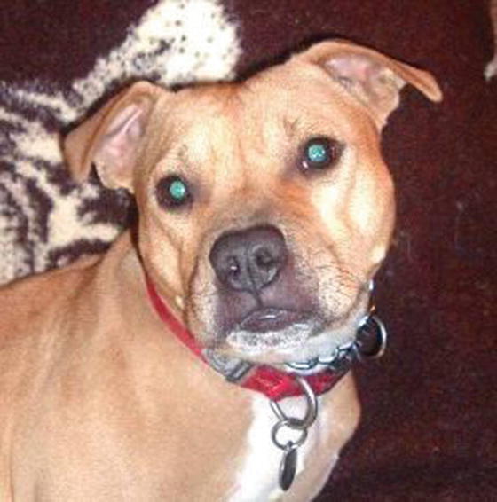
A dog image to test the accuracy of the model
- 22.Load the library and the image from the folder. You would have to change the location of the file in code snippet below.import numpy as npfrom keras.preprocessing import imagean_image =image.load_img('/Users/vaibhavverdhan/BookWriting/2.jpg',target_size =(64,64))
- 23.Let us print our final prediction.print(prediction)
The model predicts that the image is of a “dog.”
Here, in this example, we designed a Neural Network using Keras. We trained the images using images of cats and dogs and tested it. It is possible to train a multiclassifier system too if we can get the images for each of the classes.
Congratulations! You just now finished your second image classification use case using Deep Learning. Use it for training your own image datasets. It is even possible to create a multiclass classification model.
Now you may think how you will use this model to make predictions in real time. The compiled model file (e.g., 'catdog_cnn_model.h5') will be deployed onto a server to make the predictions. We will be covering model deployment in detail in the last chapter of this book.
With this, we come to the close of the second chapter. You can proceed to the summary now.
2.5 Summary
Images are a rich source of information and knowledge. We can solve a lot of business problems by analyzing the image dataset. CNNs are leading the AI revolution particularly for images and videos. They are being used in the medical industry, manufacturing, retail, BFSI, and so on. Quite a few researches are going on using CNN.
CNN-based solutions are quite innovative and unique. There are a lot of challenges which have to be tackled while designing an innovative CNN-based solution. The choice of the number of layers, number of neurons in each layer, activation functions to be used, loss function, optimizer, and so on is not a straightforward one. It depends on the complexity of the business problem, the dataset at hand, and the available computation power. The efficacy of the solution depends a lot on the dataset available. If we have a clearly defined business objective which is measurable, precise, and achievable, if we have a representative and complete dataset, and if we have enough computation power, a lot of business problems can be addressed using Deep Learning.
In the first chapter of the book, we introduced computer vision and Deep Learning. In this second chapter, we studied concepts of convolutional, pooling, and fully connected layers. You are going to use these concepts throughout your journey. And you also developed an image classification model using Deep Learning.
The difficulty level is going to increase from the next chapter onward when we start with network architectures. Network architectures use the building blocks we have studied in the first two chapters. They are developed by scientists and researchers across organizations and universities to solve complex problems. We are going to study those networks and develop Python solutions too. So stay hungry!
You should be able to answer the questions in the exercise now!
- 1.
What is the convolution process in CNN and how is the output calculated?
- 2.
Why do we need nonlinear functions in hidden layers?
- 3.
What is the difference between max and average pooling?
- 4.
What do you mean by dropout?
- 5.
Download the image data of natural scenes around the world from www.kaggle.com/puneet6060/intel-image-classification and develop an image classification model using CNN.
- 6.
Download the Fashion MNIST dataset from https://github.com/zalandoresearch/fashion-mnist and develop an image classification model.
2.5.1 Further readings
- 1.
Go through “Assessing Four Neural Networks on Handwritten Digit Recognition Dataset (MNIST)” at https://arxiv.org/pdf/1811.08278.pdf.
- 2.
Study the research paper “A Survey of the Recent Architectures of Deep Convolutional Neural Networks” at https://arxiv.org/pdf/1901.06032.pdf.
- 3.
Go through the research paper “Understanding Convolutional Neural Networks with a Mathematical Model” at https://arxiv.org/pdf/1609.04112.pdf.
- 4.
Go through “Evaluation of Pooling Operations in Convolutional Architectures for Object Recognition” at http://ais.uni-bonn.de/papers/icann2010_maxpool.pdf.