
1
From Hardware to Software
This first chapter provides a brief overview of the components found in all computers, from mainframes to the processing chips in tablets, smartphones and smart objects via desktop or laptop computers. Building on this hardware-centric presentation, we shall then give a more abstract description of the actions carried out by computers, leading to a uniform definition of the terms “program” and “execution”, above and beyond the various characteristics of so-called electronic devices.
1.1. Computers: a low-level view
Computer science is the science of rational processing of information by computers. Computers have the capacity to carry out a variety of processes, depending on the instructions given to them. Each item of information is an element of knowledge that may be transmitted using a signal and encoded using a sequence of symbols in conjunction with a set of rules used to decode them, i.e. to reconstruct the signal from the sequence of symbols. Computers use binary encoding, involving two symbols; these may be referred to as “true”/”false”, “0”/”1” or “high”/”low”; these terms are interchangeable, and all represent the two stable states of the electrical potential of digital electronic circuits.
1.1.1. Information processing
Schematically, a computer is made up of three families of components as follows:
- – memories: store data (information) and executable code (the so-called von Neumann architecture);
- – one or more microprocessors, known as CPUs (central processing units), which process information by applying elementary operations;
- – peripherals: these enable information to be exchanged between the CPU/memory couple and the outside.
Information processing by a computer – in other terms, the execution of a program – can be summarized as a sequence of three steps: fetching data, computing the results and returning them. Each elementary processing operation corresponds to a configuration of the logical circuits of the CPU, known as a logic function. If the result of this function is solely dependent on input, and if no notion of “time” is involved in the computations, then the function is said to be combinatorial; otherwise, it is said to be sequential.
For example, a binary half-adder, as shown in Figure 1.1, is a circuit that computes the sum of two binary digits (input), along with the possible carry value. It thus implements a combinatorial logic function.
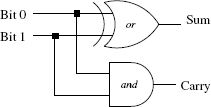
Figure 1.1. Binary half-adder
The essential character of a combinatorial function is that, for the same input, the function always produces the same output, no matter what the circumstances. This is not true of sequential logic functions.
For example, a logic function that counts the number of times its input changes relies on a notion of “time” (changes take place in time), and a persistent state between two inputs is required in order to record the previous value of the counter. This state is saved in a memory. For sequential functions, a same input value can result in different output values, as every output depends not only on the input, but also on the state of the memory at the moment of reading the new input.
1.1.2. Memories
Computers use memory to save programs and data. There are several different technologies used in memory components, and a simplified presentation is as follows:
- – RAM (Random Access Memory): RAM memory is both readable and writeable. RAM components are generally fast, but also volatile: if electric power falls down, their content is lost;
- – ROM (Read Only Memory): information stored in a ROM is written at the time of manufacturing, and it is read-only. ROM is slower than RAM, but is non-volatile, like, for example, a burned DVD;
- – EPROM (Erasable Programmable Read Only Memory): this memory is non-volatile, but can be written using a specific device, through exposure to ultra- violet light, or by modifying the power voltage, etc. It is slower than RAM, for both reading and writing. EPROM may be considered equivalent to a rewritable DVD.
Computers use the memory components of several technologies. Storage size diminishes as access speed increases, as fast-access memory is more costly. A distinction is generally made between four different types of memory:
- – mass storage is measured in terabytes and is made either of mechanical disks (with an access time of ~ 10 ms) or – increasingly – of solid-state drive (SSD) blocks. These blocks use an EEPROM variant (electrically erasable) with an access time of ~ 0.1 – 0.3 ms, known as flash memory. Mass storage is non-volatile and is principally used for the file system;
- – RAM, which is external to the microprocessor. Recent home computers and smartphones generally possess large RAM capacities (measured in gigabytes). Embedded systems or consumer development electronic boards may have a much lower RAM capacity. The access time is around 40–50 ηs;
- – the cache is generally included in the CPU of modern machines. This is a small RAM memory of a few kilobytes (or megabytes), with an access time of around 5 – 10 ηs. There are often multiple levels of cache, and access time decreases with size. The cache is used to save frequently used and/or consecutive data and/or instructions, reducing the need to access slower RAM by retaining information locally. Cache management is complex: it is important to ensure consistency between the data in the main memory and the cache, between different CPUs or different cores (full, independent processing units within the same CPU) and to decide which data to discard to free up space, etc.;
- – registers are the fastest memory units and are located in the center of the microprocessor itself. The microprocessor contains a limited number (a few dozen) of these storage zones, used directly by CPU instructions. Access time is around one processor cycle, i.e. around 1 ns.
1.1.3. CPUs
The CPU, as its name suggests, is the unit responsible for processing information, via the execution of elementary instructions, which can be roughly grouped into five categories:
- – data transfer instructions (copy between registers or between memory and registers);
- – arithmetic instructions (addition of two integer values contained in two registers, multiplication by a constant, etc.);
- – logical instructions (bit-wise and/or/not, shift, rotate, etc.);
- – branching operations (conditional, non-conditional, to subroutines, etc.);
- – other instructions (halt the processor, reset, interrupt requests,
test-and-set, compare-and-swap,etc.).
Instructions are coded by binary words in a format specific to each microprocessor. A program of a few lines in a high-level programming language is translated into tens or even hundreds of elementary instructions, which would be difficult, error prone and time consuming to write out manually. This is illustrated in Figure 1.2, where a “Hello World!” program written in C is shown alongside its counterpart in x86-64 instructions, generated by the gcc compiler.

Figure 1.2. “Hello world!” in C and in x86-64 instructions
Put simply, a microprocessor is split into two parts: a control unit, which decodes and sequences the instructions to execute, and one or more arithmetic and logic units (ALUs) , which carry out the operations stipulated by the instructions. The CPU runs permanently through a three-stage cycle:
- 1) fetching the next instruction to be executed from the memory: every microprocessor contains a special register, the Program Counter (PC), which records the location (address) of this instruction. The PC is then incremented, i.e. the size of the fetched instruction is added to it;
- 2) decoding of the fetched instruction;
- 3) execution of this instruction.
However, the next instruction is not always the one located next to the current instruction. Consider the function min in example 1.1, written in C, which returns the smallest of its two arguments.
EXAMPLE 1.1.–
Cint min (int a, int b) {if (a < b) return (a) ;else return (b) ;}
This function may be translated, intuitively and naively, into elementary instructions, by first placing a and b into registers, then comparing them:
min:load a, reg0load b, reg1compare reg0, reg1
Depending on the result of the test – true or false – different continuations are considered. Execution continues using instructions for one or the other of these continuations: we therefore have two possible control paths. In this case, a conditional jump instruction must be used to modify the PC value, when required, to select the first instruction of one of the two possible paths.
branchgt a_gt_bload reg0, reg2jump enda_gt_b:load reg1, reg2end:return reg2
The branchgt instruction loads the location of the instruction at label a_gt_b into the PC. If the result of the compare instruction is that reg0 > reg1, the next instruction is the one found at this address: load reg1, reg2. Otherwise, the next instruction is the one following branchgt: load reg0, reg2. This is followed by the unconditional jump instruction, jump, enabling unconditional modification of the PC, loading it with the address of the end label. Thus, whatever the result of the comparison, execution finishes with the instruction return reg2.
Conditional branching requires the use of a specific memory to determine whether certain conditions have been satisfied by the execution of the previous instruction (overflow, positive result, null result, superiority, etc.). Every CPU contains a dedicated register, the State Register (SR), in which every bit is assigned to signaling one of these conditions. Executing most instructions may modify all or some of the bits in the register. Conditional instructions (both jumps and more “exotic” variants) use the appropriate bit values for execution. Certain ARM® architectures [ARM 10] even permit all instructions to be intrinsically conditional.
Every program is made up of functions that can be called at different points in the program and these calls can be nested. When a function is called, the point where execution should resume once the execution of the function is completed – the return address – must be recorded. Consider a program made up of the functions g() = k() + h() and f () = g() + h(), featuring several function calls, some of which are nested.
g () =t11 = k ()t12 = h ()return t11 + t12f () =v11 = g ()v12 = h ()return v11 + v12
A single register is not sufficient to record the return addresses of the different calls. Calling k from g must be followed by calling h to evaluate t12. But this call of g was done by f, thus its return address in f should also be memorized to further evaluation of v12. The number of return addresses to record increases with the number of nested calls, and decreases as we leave these calls, suggesting very naturally to save these addresses in a stack. Figure 1.3 shows the evolution of a stack structure during successive function calls, demonstrating the need to record multiple return addresses. The state of the stack is shown at every step of the execution, at the moment where the line in the program is being executed.
A dedicated register, the Stack Pointer (SP), always contains the address of the next free slot in the stack (or, alternatively, the address of the last slot used). Thus, in the case of nested calls, the return address is saved at the address indicated by the SP, and the SP is incremented by the size of this address. When the function returns, the PC is loaded with the saved address from the stack, and the SP is decremented accordingly.

Figure 1.3. Function calls and return addresses
In summary, the internal state of a microprocessor is made up of its general registers, the program counter, the state register and the stack pointer. Note, however, that this is a highly simplified vision. There are many different varieties of microprocessors with different internal architectures and/or instruction sets (for example, some do not possess an integer division instruction). Thus, a program written directly using the instruction set of a microprocessor will not be executable using another model of microprocessor, and it will need to be rewritten. The portability of programs written in the assembly language of a given microprocessor is practically null. High-level languages respond to this problem by providing syntactic constructs, which are independent of the target microprocessors. The compiler or the interpreter have to translate these constructs into the language used by the microprocessor.
1.1.4. Peripheral devices
As we saw in section 1.1.3, processors execute a constant cycle of fetching, decoding and executing instructions. Computations are carried out using data stored in the memory, either by the program itself or by an input/output mechanism. The results of computations are also stored in the memory, and may be returned to users using this input/output mechanism.
The interest of any programmable system is inherently dependent on input/output capacities through which the system reacts to the external environment and may act on this environment. Even an assembly robot in a car factory, which repeats the same actions again and again, must react to data input from the environment. For example, the pressure of the grip mechanism must stop increasing once it has caught a bolt, and the time it takes to do this will differ depending on the exact position of the bolt.
Input/output systems operate using peripherals, ancillary devices that may be electronic, mechanical or a combination of the two. These allow the microprocessor to acquire external information, and to transmit information to the exterior. Computer mice, screens and keyboards are peripherals used with desktop computers, but other elements such as motors, analog/digital acquisition cards, etc. are also peripherals.
If peripherals are present, the microprocessor needs to devote part of its processing time to data acquisition and to the transmission of computed results. This interaction with peripherals may be directly integrated into programs. But in this case, the programs have to integrate regular checking of input peripherals to see if new information is available. It is technically difficult (if not impossible) to include such a monitoring in every program. Furthermore, regular peripheral checks are a waste of time and energy if no new data is available. Finally, there is no guarantee that information would arrive exactly at the moment of checking, as data may be asynchronously emitted.
This problem can be avoided by relying on the hardware to indicate the occurrence of new external events, instead of using software to check for these events. The interrupt mechanism is used to interrupt the execution of the current code and to launch the interrupt handler associated with the external event. This handler is a section of code, which is not explicitly called by the program being executed; it is located at an address known by the microprocessor. As any program may be interrupted at any point, the processor state, and notably the registers, must be saved before processing the interrupt. The code that is executed to process the interrupt will indeed use the registers and modify the SR, SP and PC. Therefore, previous values of registers must be restored in order to resume execution of the interrupted code. This context saving is carried out partially by the hardware and partially by the software.
1.2. Computers: a high-level view
The low-level vision of a von Neumann machine presented in section 1.1 provides a good overview of the components of a computer and of program execution, without going into detail concerning the operations of electronic components. However, this view is not particularly helpful in the context of everyday programming activity. Programs in binary code, or even assembly code, are difficult to write as they need to take account of every detail of execution; they are, by nature, long and hard to review, understand and debug. The first “high-level” programming languages emerged very shortly after the first computers. These languages assign names to certain values and addresses in the memory, providing a set of instructions that can be split into low-level machine instructions. In other terms, programming languages offer an abstract vision of the computer, enabling users to ignore low-level details while writing a program. The “hello world” program in Figure 1.2 clearly demonstrates the power of abstraction of C compared to the X86 assembly language.
1.2.1. Modeling computations
Any program is simply a description, in its own programming language, of a series of computations (including reading and writing), which are the only operations that a computer can carry out. An abstract view of a computer requires an abstract view – we call it a model – of the notion of computation. This subject was first addressed well before the emergence of computers, in the late 19th century, by logicians, mathematicians and philosophers, who introduced a range of different approaches to the theory of calculability.
The Turing machine [TUR 95] is a mathematical model of computation introduced in 1936. This machine operates on an infinite memory tape divided into cells and has three instructions: move one cell of the tape right or left, write or read a symbol in the cell or compare the contents of two cells. It has been formally proven that any “imperative” programming language, featuring assignment, a conditional instruction and a while loop, has the same power of expression as this Turing machine.
Several other models of the notion of algorithmic computation were introduced over the course of the 20th century, and have been formally proven to be equivalent to the Turing machine. One notable example is Kleene’s recursion theory [KLE 52], the basis for the “pure functional” languages, based on the notion of (potentially) recursive functions; hence, these languages also have the same power of expression as the Turing machine. Pure functional and imperative languages have developed in parallel throughout the history of high-level programming, leading to different programming styles.
1.2.2. High-level languages
Broadly speaking, the execution of a functional program carries out a series of function calls that lead to the result, with intermediate values stored exclusively in the registers. The execution of an imperative program carries out a sequence of modifications of memory cells named by identifiers, the values in the cells being computed during execution. The most widespread high-level languages include both functional and imperative features, along with various possibilities (modules, object features, etc.) to divide source code into pieces that can be reused.
Whatever the style of programming used, any program written in a high-level language needs to be translated into binary language to be executed. These translations are executed either every time the program is executed – in which case the translation program is known as an interpreter or just once, storing the produced binary code – in which case the translator is known as a compiler.
As we have seen, high-level languages facilitate the coding of algorithms. They ease reviewing of the source code of a program, as the text is more concise than it would be for the same algorithm in assembly code. This does not, however, imply that users gain a better understanding of the way the program works. To write a program, a precise knowledge of the constructs used – in other terms, their semantics, what they do and what they mean – is crucial to understand the source code. Bugs are not always the result of algorithm coding errors, and are often caused by an erroneous interpretation of elements of the language. For example, the incrementation operator ++ in C exists in two forms (i++ or ++i), and its understanding is not as simple as it may seem. For example, the program:
C#include <stdio.h>int main () {int i = 0 ;printf (“%d ”, i++) ;return (0) ;}
will print 0, but if i++ is replaced with ++i, the same program will print 1.
There are a number of concepts that are common to all high-level languages: value naming, organization of namespaces, explicit memory management, etc. However, these concepts may be expressed using different syntactic constructs. The field of language semantics covers a set of logico-mathematical theories, which describe these concepts and their properties. Constructing the semantics of a program allows to the formal verification of whether the program possesses all of the required properties.
1.2.3. From source code to executable programs
The transition from the program source to its execution is a multistep process. Some of these steps may differ in different languages. In this section, we shall give an overview of the main steps involved in analyzing and transforming source code, applicable to most programming languages.
The source code of a program is made up of one or more text files. Indeed, to ease software architecture, most languages allow source code to be split across several files, known as compilation units. Each file is processed separately prior to the final phase, in which the results of processing are combined into one single executable file.
1.2.3.1. Lexical analysis
Lexical analysis is the first phase of translation: it converts the sequence of characters that is indeed the source file into a sequence of words, assigning each to a category. Comments are generally deleted at this stage. Thus, in the following text presumed to be written in C
/* This is a comment. */if [x == 3 int +) cos ($v)
lexical analysis will recognize the keyword if, the opening bracket, the identifier x, the operator ==, the integer constant 3, the type identifier int, etc. No word in C can contain the character $, so a lexical error will be highlighted when $v is encountered.
Lexical analysis may be seen as a form of “spell check”, in which each recognized word is assigned to a category (keyword, constant, identifier). These words are referred to as tokens.
1.2.3.2. Syntactic analysis
Every language follows grammar. For example, in English, a sentence is generally considered to be correctly formed if it contains a subject, verb and complement in an understandable order. Programming languages are no exception: syntactic analysis verifies that the phrases of a source file conform with the grammar of their language. For example, in C, the keyword if must be followed by a bracketed expression, an instruction must end with a semicolon, etc. Clearly, the source text given in the example above in the context of lexical analysis does not respect the syntax of C.
Technically, the syntactic analyzer is in charge of the complete grammatical analysis of the source file. It calls the lexical analyzer every time it requires a token to progress through the analyzed source. Syntactic analysis is thus a form of grammar verification, and it also builds a representation of the source file by a data structure, which is often a tree, called the abstract syntax tree (AST). This data structure will be used by all the following phases of compilation, up to the point of execution by an interpreter or the creation of an executable file.
1.2.3.3. Semantic analyses
The first two analysis phases of compilation only concern the textual structure of the source. They do not concern the meaning of the program, i.e. its semantics. Source texts that pass the syntactic analysis phase do not always have meaning. The phrase “the sea eats a derivable rabbit” is grammatically correct, but is evidently nonsense.
The best-known semantic analysis is the typing analysis, which prohibits the combination of elements that are incompatible in nature. Thus, in the previous phase, “derivable” could be applicable to a function, but certainly not to a “rabbit”.
Semantic analyses do not reduce to a form of typing analysis but they all interpret the constructs of a program according to the semantics of the chosen language. Semantic analyses may be used to eliminate programs, which leads to execution errors. They may also apply some transformations to program code in order to get an executable file (dependency analysis, closure elimination, etc.). These semantic analyses may be carried out during subsequent passes of source code processing, even after the code generation phase described in the following section.
1.2.3.4. Code interpretation/generation
Once the abstract syntax tree (or a derived tree) has been created, there are two options. Either the tree may be executed directly via an interpreter, which is a program supplied by the programming language, or the AST is used to generate object code files, with the aim of creating an executable file that can be run independently. Let us first focus on the second approach. The interpretation mechanism will be discussed later.
Compilation uses the AST generated from the source file to produce a sequence of instructions to be executed either by the CPU or by a virtual machine (VM). The compilation is correct if the execution of this sequence of instructions gives a result, which conforms to the program’s semantics.
Optimization phases may take place during or after object code generation, with the aim of improving its compactness or its execution speed. Modern compilers implement a range of optimizations, which study lies outside the scope of this book. Certain optimizations are “universal”, while others may be specific to the CPU for which the code is generated.
The object code produced by the compiler may be either binary code encoding instructions directly or source text in assembly code. In the latter case, a program – known as the assembler – must be called to transform this low-level source code into binary code. Generally speaking, assemblers simply produce a mechanical translation of instructions written mnemonically (mov, add, jmp, etc.) into binary representations. However, certain more sophisticated assemblers may also carry out optimization operations at this level.
Assembling mnemonic code into binary code is a very simple operation, which does not alter the structure of the program. The reference manual of the target CPU provides, for each instruction, the meaning of the bits of the corresponding binary word. For example, the reference manual for the MIPS32® architecture [MIP 13] describes the 32-bit binary format of the instruction ADD rd, rs, rt (with the effect rd ← rs + rt on the registers) as:

Three packets of 6 bits are reserved for encoding the register numbers; the other bits in this word are fixed and encode the instruction. The task of the assembler is to generate such bit patterns according to the instructions encountered in the source code.
1.2.3.5. Linking
A single program may be made up of several source files, compiled separately. Once the object code from each source file has been produced, all these codes must be collected into a single executable file. Each object file includes “holes”, indicating unknown information at the moment of production of this object code. It is important to know where to find this missing code, when calling functions defined in a different compilation unit, or where to find variables defined in a location outside of the current unit.
The linker has to gather all the object files and fill all the holes. Evidently, for a set of object files to lead to an executable file, all holes must be filled; so the code of every function called in the source must be available. The linking process also has to integrate the needed code, if it comes from some libraries, whether from the standard language library or a third-party library. There is one final question to answer, concerning the point at which execution should begin. In certain languages (such as C, C++ and Java), the source code must contain one, and only one, special function, often named main, which is called to start the execution. In other languages (such as Python and OCaml), definitions are executed in the order in which they appear, defined by the file ordering during the linking process. Thus, “executing” the definition of a function does not call the function: instead, the “value” of this function is created and stored to be used later when the function is called. This means that programmers have to insert into the source file a call to the function which they consider to be the “starting point” of the execution. This call is usually the final instruction of the last source file processed by the linker.
A simplified illustration of the different transformation passes involved in source code compilation is shown in Figure 1.5.

Figure 1.5. Compilation process
1.2.3.6. Interpretation and virtual machines
As we have seen, informally speaking, an interpreter “executes” a program directly from the AST. Furthermore, it was said that the code generation process may generate code for a virtual machine. In reality, interpreters rarely work directly on the tree; compilation to a virtual machine is often carried out as an intermediate stage. A virtual machine (VM) may be seen as a pseudo-microprocessor, with one or more stacks, registers and fairly high-level instructions. The code for a VM is often referred to as bytecode. In this case, compilation does not generate a file directly executable by the CPU. Execution is carried out by the virtual machine interpreter, a program supplied by the programming language environment. So, the difference between interpretation and compilation is not clear-cut.
There are several advantages of using a VM: the compiler no longer needs to take the specificities of the CPU into account, the code is often more compact and portability is higher. As long as the executable file for the virtual machine interpreter is available on a computer, it will be possible to generate a binary file for the computer in question. The drawback to this approach is that the programs obtained in this way are often slower than programs compiled as “native” machine code.