6
MICROWAVE BACKHAUL NETWORKS
6.1 INTRODUCTION
Microwave radios play a key role in today’s telecommunication networks and are much more common than many may suspect. Though sometimes hidden from the eye, point-to-point (PtP) microwave radios make up almost half of the cellular backhaul connections worldwide and comprise more than two-thirds of worldwide connections outside of the United States.
Radios are also common in carriers’ long-haul connections and metropolitan networks serving as fiber replacements. Private enterprise networks, public safety and military networks, and utility companies are also utilizing microwave systems. Still, the most common deployment scenario of PtP radios remains the backhauling of cellular networks.
When talking about mobile backhaul, let us have a look on the market size and its growth: The number of worldwide mobile subscribers was 3.3 billion in 2007 and will grow to 5.2 billion by 2011. According to a report by Infonetics Research, the number of backhaul connections is expected to grow from 2.6 million in 2007 to 4.3 million by 2011.
The microwave radio is so widely deployed mainly because fiber cannot be made available everywhere. In addition, microwave makes for fast and cost-effective deployment compared to fiber. In many cases, self-build and ownership of microwave is cheaper than leasing fiber or copper T/E lines from the incumbent carrier. The new offering of microwave radios supporting carrier Ethernet specifically suits the needs of the growing mobile backhaul, which is pushed into Ethernet technology nowadays.
New mobile technologies such as 3G, WiMAX, and LTE deliver high data rates and lead to a rapid increase in bandwidth-consuming applications. This requires operators to significantly expand their networks or to risk not being able to provide an adequate service quality. The main problem facing operators today is that the demand for bandwidth is not accompanied by a proportional revenue growth. Users demand data bandwidth but are not willing to pay a premium for it as they have for voice services. Instead, they expect a flat-rate model like they get for their residential high-speed data services like DSL or cable. Considering this problem, the cost of expansion of legacy networks becomes unacceptable and operators are forced to move toward new solutions based on the more cost-efficient carrier Ethernet.
The carrier Ethernet represents the only viable solution because it brings the cost model of Ethernet to mobile backhaul. Certainly the technology also has some risks, for instance, supporting legacy networks and the key element of clock synchronization required by mobile applications. Be that as it may, many analysts agree that the number of cell sites served by an Ethernet backhaul will continue to expand rapidly. Analyst group Heavy Reading [2,3] claims that in 2008 only 23,000 cell sites worldwide were served with Ethernet, about 1% of the total ∼2 million. This figure is expected reach to 713,000 by the end of 2012, or 24% of the total ∼3 million.
As mobile services become more and more sophisticated, and considering a widely spreading trend of convergence with fixed networks, operators need to do more than simply deliver basic voice and best-effort data. For this they need the tools to differentiate their services, and they need to integrate those tools into the transport layer. The new microwave radios are much more than transport “pipes.” Integrating advanced functionality such as service differentiation and policy enforcement tools is needed in order to achieve successful and profitable backhaul deployment.
Microwave radios offered today include a wide selection of legacy transport radios, such as (a) carrier Ethernet radios and (b) hybrid radios supporting both legacy and Ethernet technologies that allow for smooth migration from legacy to next-generation networks [4].
In this chapter we will review the microwave radio technology and focus specifically on (a) point-to-point radio applications for mobile backhaul and (b) the way it evolves today for supporting the rapidly growing cellular networks.
The first part of the chapter will go through some fundamental radio techniques and will compare various types of this technology, including point-to-point versus point-to-multipoint radios. The second part of the chapter will focus on networking features and attributes of modern radios, primarily explaining Ethernet radio technology and what is required for such radios for carrier Ethernet backhaul. The final section will be dedicated to mobile backhaul evolution challenges and possible solution alternatives.
6.2 MICROWAVE RADIO FUNDAMENTAL TECHNIQUES
6.2.1 Radio Link Budget, System Gain, and Availability
Radio link budget is a basic calculation that is essential for any radio deployment [5]. In order to maintain a radio link, the received signal level at each receiver should be above a threshold level that ensures the minimum signal-to-noise ratio (SNR) and enables the receiver to lock on the signal and demodulate it successfully. This threshold level is typically measured at a bit error rate (BER) of 10−6, denoted as Pth. BER level depends on the radio modulation scheme, modem implementation (such as coding strength and modem quality), and radio implementation factors such as noise figure, branching losses from the antenna, and other losses.
The received signal strength can be calculated as follows:
![]()
where PRX is the received signal level, PTX is the transmitted power level, GTX and GRX are the transmitting and receiving antenna gain, FSL is the free-space propagation loss (proportional to 1/R2, where R is the link distance, as well as to 1/f 2, where f is the link frequency), and L represents additional losses caused by many factors such as atmosphere gas absorption, rain fading, or obstacles.
The fade margin of a given link, with a given threshold, refers to the maximum loss (L) at which the link still delivers data at the specified BER:
![]()
The term PTX − PTH is usually referred to as system gain.
![]()
The system gain is a commonly used figure of merit for comparing the performance of different competing radio systems. A radio with higher system gain will have a higher fade margin, allowing it to be used over a longer link distance or in combination with smaller (less expensive) antennas compared with other lower system gain radios.
Radio Availability.
Availability is defined in terms of percentage of yearly time of service and is calculated as 100% of the time minus the annual outage time in which traffic loss occurs. For example, availability of 99.999%, sometimes referred to as “five 9’s,” means that the expected traffic loss is not more than 0.001% of the time in a year, which is approximately 5 minutes a year.
Unlike wireline applications, radio networks are designed to deal with expected outages. While in wireline networks a link breakdown (such as fiber cut) is obviously a failure mode, in wireless radio links, a link breakdown due to channel fades is simply one more scenario that needs to be planned for. Correct planning for specific service level objective enables operators to rely on their microwave network with just the same confidence as with wired network.
Rain Fade Margin and Availability.
The main cause for radio link fades is rain attenuation. The more intense the rain is (as measured in millimeters/hour), the more it attenuates the propagating signal, with exponential dependency. Other precipitation forms such as snow or fog do not cause significant propagation loss at the microwave frequencies (unlike optical systems for example, which are severely affected by fog). Rain attenuation increases significantly in frequency and also varies in polarization. Since falling rain drops are not shaped as spheres, the horizontal polarization is attenuated more than vertical polarization. It should be noted that at low frequencies (below 8 GHz), rain attenuation may not be the dominant outage factor, but rather multipath effects resulting from reflections. This will be described further in the chapter when we discuss diversity.
Link fade margin planning is based on statistical distribution models that measure rain intensity. These models rely on historical rain measurements, and they divide the globe into “rain zones.”
The two commonly used models for calculating rain-fade margin are the ITU-R and Crane models. Both allow planners to compute the required fade margin for a given radio link frequency, link length, and rain zone, in order to reach the desired availability. It should be noted that rain effects result from the actual blockage of the radio path by heavy rain cells. Once this happens, neither equipment nor antenna redundancy can help to overcome the blockage. On the other hand, because heavy rain usually occurs within relatively small areas at a given time, path diversity may help. By using redundant path topologies such as a ring, operators can maintain their services on a network level even when a particular radio path is temporarily blocked.
6.2.2 Multipath Fading and Radio Diversity
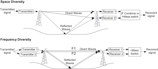
As mentioned above, rain fading is less severe in lower frequencies, but multipath fading becomes more dominant. Multipath fading results from the reflected waves reaching the receiver and mixing with the desired signal at random phases, as shown in Figure 6.1.
Figure 6.1. Radio diversity systems.
Multipath fading depends mainly on the link geometry and is more severe at long-distance links and over flat surfaces or water. Multipath fading is also affected by air turbulence and water vapor, and it can vary quickly during temperature changes due to rapid changes in the reflections phase.
It is common to distinguish between flat fading, which equally affects the entire channel bandwidth, and selective fading, which is frequency-dependent over the given channel bandwidth.
The common way to handle severe multipath conditions is to use diversity techniques, mainly space or frequency diversity, as shown at Figure 6.1.
Multipath fading depends on geometry. So if we place two receivers (with separate antennas) at a sufficient distance from one another, multipath fading will become uncorrelated between both receivers. Thus, statistically, the chance for destructive fading at both ends decreases significantly. Frequency diversity uses a single antenna and two simultaneous frequency channels. While both diversity solutions require a second receiver, space diversity also requires a second antenna. On the other hand, frequency diversity requires double the spectrum usage (this is generally less favored by regulators).
With space diversity there are two options to recover the signal. One is through hitless switching, where each receiver detects its signal independently, but the output is selected dynamically from the best one. Switching from one receiver to the other must be errorless. Another signal recovery option is to combine both signals in phase with each other to maximize the signal-to-noise ratio. IF combining, as it is commonly referred to, is usually handled by analog circuitry at the intermediate frequency (IF). This way is much better because the in-phase combining of both signals can cancel the notches at both received signals and thus increase significantly the dispersive fade margin, as well as increase the system gain up to 3 dB with flat fading.
With frequency diversity, as the different signals are carried over different carrier waves, IF combining is not possible but only hitless switching is relevant.
6.2.3 Modulation, Coding, and Spectral Efficiency
Microwave radio is based on transmitting and receiving a modulated electromagnetic carrier wave. At the transmit side, the modulator is responsible for conveying the data on the carrier wave. This is done by varying its amplitude, frequency, or phase. At the receive side, the demodulator is responsible for synchronizing on the receive signal and reconstructing the data. Legacy radio systems implemented simple analog modulation schemes. One such scheme is frequency shift keying (FSK), where for each time period T, the symbol time, one of several carrier frequencies was selected. Modern radios use digital modulators that allow much higher numbers of amplitude and phase possible states for each symbol, usually from 4 QAM (QPSK) up to 256 QAM. The more states the modulation has, the more data it can carry over one symbol. For example, QPSK has four possible states and thus carries 2 bits/symbol, whereas 256 QAM carries 8 bits/symbol.
The channel bandwidth that is occupied by the transmitted signal depends on the symbol rate, which is 1/T (where T is the symbol time), and on the signal filtering following the modulator. Hence, for a given channel bandwidth, there is a limited symbol rate that the radio can use, and consequently there is a limited data rate that it can transmit.
Let us now look at the following example. ETSI [11,12] defines for most frequency bands a channel separation of 1.75 MHz to 56 MHz. ETSI also defines a spectrum mask for each channel and modulation to guarantee a certain performance of spectral emissions and interferences of adjacent and second adjacent channels. A modern digital radio system can usually utilize a symbol rate of 50 MHz over a 56-MHZ channel, and thus it can deliver 400 Mbit/s by using 256 QAM modulation.
Modern digital radios also use error correction coding that requires parity bits to be added to the information bits. The term coding rate is used to define the portion of net data bits out of the total number of bits. For instance, a coding rate of 0.95 means that out of each 100 bits transmitted, 95 are the “useful” information bits. A stronger code will use more parity bits, and thus it will have a lower rate. In addition, part of the symbols may be used for synchronization purposes and not for carrying data.
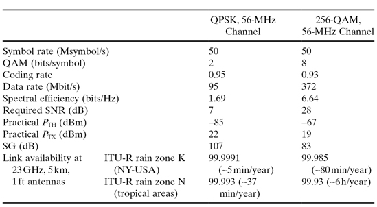
Now that we can compute the net data rate provided by a radio system, we can go on to monitor its spectral efficiency. The term spectral efficiency refers to the number of information bits that are carried over 1 Hz of spectrum. If we now take again the above example of 256 QAM over 56 MHz and assume a coding rate of 0.93, we get the net data rate of 372 Mbps and obtain a spectral efficiency of 6.64 bits/Hz, as shown in Table 6.1.
TABLE 6.1. System Gain and Availability Examples
Since bandwidth is a precious resource, with massive demand and growth in high capacity radio deployments, regulators today encourage the deployment of high spectral efficiency systems and sometimes even requires a certain minimal efficiency.
The Tradeoffs of Spectral Efficiency.
When calculating spectral efficiency, we need to consider the required system gain and the system’s complexity and cost.
System Gain.
As a general rule, higher spectral efficiency means lower system gain and therefore poor availability. The information theory bounds the information rate that can be delivered over a given channel with a given signal-to-noise ratio (SNR). This is defined by the well-known Shannon formula: C = W log 2(1 + SNR), where C is channel capacity in bits/hertz and W is channel bandwidth in hertz. Note that C/W just equals spectral efficiency. From the Shannon formula we can clearly understand that in order to have higher spectral efficiency, we need a better SNR to demodulate the signal and restore the information successfully. The formula shows that at higher SNRs each increase of 1 bit/Hz will require doubling the SNR—that is, improve it by 3 dB. The need for higher SNR means higher thresholds and results in lower system gain, both of which translate into lower availability (under the same other link conditions).
System Complexity.
Implementation of higher efficiency modulations involves an increasing cost and complexity for both the transmitter and the receiver. Higher modulations require lowering the quantization noise. This in turn will require higher-precision analog-to-digital and digital-to-analog converters, along with much more digital hardware for performing all digital processing at a higher precision. As higher modulation schemes become much more sensitive to signal distortion, they require better linearity and phase noise of the analog circuitry, as well as additional complex digital processing (such as longer equalizers) to overcome such distortions. Additionally, the requirement for linearity typically means that by using the same power amplifier, a system can obtain less transmit power at a higher modulation, so system gain is decreased twice: one time due to higher SNR and another time due to lower PTX.
The selection of one system or another depends on the specific requirements of the operator and restrictions (or lack thereof) of the regulator. Luckily, many modern radio systems are software-defined, so one piece of equipment can be configured to different working modes according to user preferences.
The example in Table 6.1 compares two modern radio systems and shows the tradeoff between system gain and spectral efficiency. As can be seen in the table, the 256 QAM system delivers almost four times the capacity of the QPSK system, but has a SG lower by 24 dB! Given the same link conditions, we can also see the difference in availability between the systems, which is very significant especially at high rain rate zones such as ITU-R zone N.
A Word About Error Correction Codes.
We have mentioned briefly the option to use some transmitted bits as parity bits to allow error correction and robust delivery of information bits. We’ve also mentioned the Shannon formula, which sets the theoretical limit for channel capacity within a given SNR. When Shannon’s formula was published in 1948, there was no implementation foreseen that was, or would be, able to get near its limit. Over the years, implementations of codes such as Reed–Solomon became very common in radio design, enabling systems to reach within a few decibels of Shannon’s limit. More recent techniques, such as turbo codes or low-density-parity-check (LDPC) codes, come even closer to reaching the theoretical Shannon limit—at times as close as only a few tenths of a decibel. Such codes require a very high computational complexity, but the advances in silicon processes have made them practical (even at very high bit rates) and allow them to be implemented in state-of-the-art radios today.
Enhancing Spectral Efficiency with XPIC.
One way to break the barriers of spectral efficiency is to use dual-polarization radio over a single-frequency channel. A dual polarization radio transmits two separate carrier waves over the same frequency, but using alternating polarities. Despite its obvious advantages, one must also keep in mind that typical antennas cannot completely isolate the two polarizations, and isolation better than 30 dB is hard to achieve. In addition, propagation effects such as rain can cause polarization rotation, making cross-polarization interferences unavoidable. The relative level of interference is referred to as cross-polarization discrimination (XPD). While lower spectral efficiency systems (with low SNR requirements such as QPSK) can easily tolerate such interferences, higher modulation schemes cannot and require cross-polarization interference canceler (XPIC). The XPIC algorithm allows detection of both streams even under the worst levels of XPD such as 10 dB. This is done by adaptively subtracting from each carrier the interfering cross carrier, at the right phase and level. For high-modulation schemes such as 256 QAM, an improvement factor of more than 20 dB is required so that cross-interference does not limit performance anymore. XPIC implementation involves system complexity and cost since the XPIC system requires each demodulator to cancel the other channel interference.
XPIC radio may be used to deliver two separate data streams, such as 2xSTM1 or 2xFE, as shown at Figure 6.2a. But it can also deliver a single stream of information such as gigabit Ethernet, or STM-4, as shown at Figure 6.2b. The latest case requires a demultiplexer to split the stream into two transmitters, and it also needs a multiplexer to join it again in the right timing because the different channels may experience a different delay. This system block is called “multi-radio,” and it adds additional complexity and cost to the system.
Figure 6.2. (a) XPIC system delivering two independent data streams. (b) XPIC system delivering a single data stream (multi-radio).
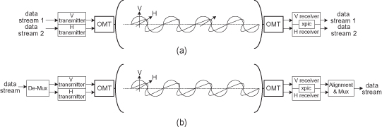
It should be noted that there are different techniques regarding how to split the traffic between radios. For example, Ethernet traffic can be divided simply by using standard Ethernet link aggregation (LAG), but this way is not optimal. Since LAG divides traffic-based flow basis, it will not be divided evenly, and it can even be that all traffic is on a single radio, thus not utilizing the second radio channel. A more complex but optimal way is to split the data at the physical layer, taking each other bit or byte to a different radio, so all radio resources are utilized.
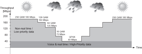
Adaptive Modulation.
Adaptive modulation means dynamically varying the modulation in an errorless manner in order to maximize throughput under momentary propagation conditions. In other words, a system can operate at its maximum throughput under clear sky conditions and can decrease it gradually under rain fade [26].
Legacy microwave networks based on PDH or SDH/SONET deliver a fixed, “all or nothing” pipe of information and cannot accommodate for any reduction in the link’s capacity. This can be further explained by the following example. An STM-1/OC-3 radio link with 155.52-Mbit/s capacity is carried over a radio link using a 28-MHz channel. In this case, a modulation of 128 QAM is required, with a typical SNR threshold of ∼25 dB. Let us now suppose that a short fade occurs, causing the SNR to drop by 2 dB below this threshold. Should this happen, the connection fails entirely, since the SDH equipment will not be able to tolerate either the errors or any decrease in throughput. Unlike legacy networks, emerging packet networks allow the link to simply lower the modulation scheme under the conditions described above. In this particular case, dropping the modulation to 64 QAM will decrease the capacity to approximately 130 Mbps but will not cause the link to fail and will continue to support the service.
An adaptive QAM radio can provide a set of working points at steps of approximately 3 dB. This results from the modulation scheme change, since the SNR threshold changes by 3 dB for each additional bit per hertz. For “finer” steps, it is also possible to change the coding scheme [adaptive coding and modulation (ACM)]. This may further increase throughput by as much as 10%. System performance can be further enhanced by combining adaptive modulation with adaptive power control. As we have already seen, a lower modulation scheme usually allows higher power levels due to relaxed linearity requirements. Hence an additional increase in system gain can be achieved when reducing the modulation scheme and simultaneously increasing the transmitted power.
It should be noted that adaptive radios are subject to regulatory authorization. ETSI standards were recently adopted to allow such systems, and a similar process has begun by the FCC. Still, not all local regulators allow it.
An example for ACM system with five working points is shown in Table 6.2, demonstrating the range of system gain versus throughput and also showing a test case of availability difference over this range. Figure 6.3 shows the behavior over time of such system under a severe fade situation.
TABLE 6.2. ACM Example
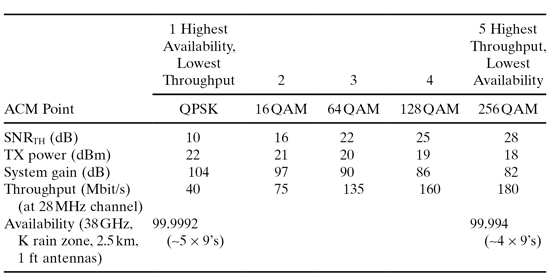
Figure 6.3. ACM example.
6.3. DIFFERENT TYPES OF RADIO TECHNOLOGIES
Modern telecommunication networks employ a variety of radio technologies. All of these technologies involve transmitting radio waves between two or more locations, but they also differ a lot from one another both in the method of transmission and in the application they are best suited for. The lion’s share of this chapter will focus on point-to-point (PtP) radios over licensed frequencies that make up for more than 90% of wireless backhaul solutions today. In addition, we will describe several other technologies, considering the pros and cons of each one.
6.3.1 Point-to-Point and Point-to-Multipoint Radios
A point-to-point (PtP) radio link consists of two symmetrical terminals transmitting and receiving signals between the two sites. A point-to-multipoint (PtMP) system, on the other hand, contains a central site (sometimes called “hub”) that is connected to number of remote terminals.
Let us now consider the advantages and disadvantages of PtP and PtMP architectures. The example depicted in Figure 6.4 shows a hub site connected to four edge sites by using four PtP radio links, or one PtMP 90 ° sector serving the four users.
Figure 6.4. PtP and PtMP.
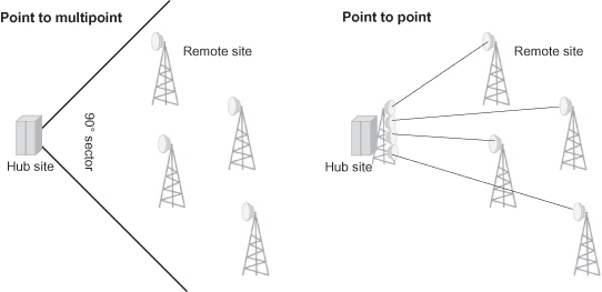
Using a pure equipment-count comparison, it’s plain to see that PtMP has an edge. The PtMP sector will require 4 + 1 equipment units and antennas, whereas the equivalent PtP solution requires 2 × 4 units and antennas. But equipment count may not be the only consideration, and we should also look at the radio link budget.
Since the PtMP sector antenna has a very wide beam width as compared to the PtP link that uses two directional antennas, PtP will have a significant advantage in system gain. Thus higher capacities can be delivered, or, in turn, an operator can use lower-power and smaller antennas to achieve similar results as in PtMP. For example, a typical sector antenna gain is 10–15 dBi, whereas a typical gain of a PtP antenna in use today is around 40 dBi and even higher. So, assuming that the remote radio antenna is identical, the difference in system gain can be around 30 dB in favor of PtP. This big difference is a major limit in reaching high capacities with high availably using PtMP radios.
Another major difference between the PtP and PtMP is the use of the radio-frequency spectrum as a shared media versus dedicated media. The PtMP sector shares the same frequency channel among several users to allow more flexibility and enable statistical multiplexing between users. The use of a dedicated channel for each PtP link, however, does not allow using excess bandwidth of one user and pass it to another. Shared media PtMP also offers the benefit of statistical multiplexing; but in order to enjoy it, operators must deploy a wide sector antenna that has a downside of interferences between other links at the same channel, thus poor spectrum reuse. In contrast, PtP antennas make it easier to reuse frequency channels while avoiding interferences from one radio link to another due to its pencil beam antennas.
The wide-angle coverage of PtMP makes frequency planning more complex and limited, and frequency reuse is not trivial and hard to regulate with interferences between different hubs, especially with large coverage deployments such as mobile backhaul. Therefore it is uncommon to find PtMP architecture in these applications, unlike radio access networks asWiMAX where PtMP is more commonplace.
6.3.2 Line of Sight and Near/No Line of Sight Radios
The segmentation of line of sight (LOS) and near/no line of sight (NLOS) radios goes hand in hand with the frequency segmentation of above and below 6 GHz. For high-frequency radios, an LOS between the radios is generally required and the accepted criteria for LOS is usually defined as keeping the first Fresnel zone clear of any obstacles. Such clearance allows radio waves to propagate across an uninterrupted path, while any obstacle on the way (which can be any physical object of conducting or absorbing materials like trees, buildings, and ground terrain) will cause attenuations, reflections, and diffractions of the signal. The ability to maintain a radio connection under such conditions decreases as the frequency increases.
NLOS communication typically refers to frequencies up to 6 GHz. Unlike LOS propagation in which signal level decrease over distance R is proportional to (1/R)2, NLOS signal level decreases faster, proportional to a higher order of 1/R. Hence the connection distance is decreased significantly, depending on link obstacles and terrain. In addition, NLOS connections require radio capability to handle signal distortions and interferences resulting from the NLOS propagation (such as OFDM modems), which are not trivial to implement—especially with high-bandwidth signals and high spectral efficiency modulation.
Most access technologies today including cellular, WiFi, and Wimax handle NLOS connections as a matter of definition. NLOS backhaul can make for easier and cheaper deployment, since LOS is not always possible or available and can require high-cost construction of antenna towers.
Still, NLOS has a number of major drawbacks when compared to LOS:
- Limited Available Spectrum. Sub-6-GHz bands are limited. Most licensed bands in this range are assigned to access applications (e.g., cellular, Wimax) and are therefore expensive to purchase. Unlicensed bands (such as WiFi) are congested and unreliable for backhaul usage.
- Limited Capacity. NLOS propagation and low-gain antennas limit traffic capacities that cannot compete with those of high frequencies.
- Complicated Planning. Complicated planning and the inability to accurately predict propagation and interferences make it very difficult to guarantee a robust backhaul network with carrier-grade availability.
6.3.3 Licensed and Unlicensed Radios
This is a regulative aspect of microwave radios that needs to be mentioned. Most countries consider spectrum a national resource that needs to be managed and planned. Spectrum is managed at a global level by the UN’s International Telecommunication Union (ITU), at a regional level by bodies such as the European Conference of Postal and Telecommunications Administrations, and at national levels by agencies such as the Office of Communication (OFCOM) in the United Kingdom or the Federal Communication Commission (FCC) in the United States.
The implications of using a licensed spectrum radio are simple to understand: The operator must pay the toll, and in return he is guaranteed that no interferences from other licensed operators will harm the radio performance. For the backhaul network designer, such a guarantee is crucial for guaranteeing his service level.
The nature of the license differs from country to country and between frequency bands. For example, some licenses cover specific channels (usually paired as “go” and “return” channels), while others cover a bulk frequency (such as LMDS); licenses can be given for nationwide transmission, whereas others are given for a single radio link only; and regulators might license the channel at both polarizations separately, or they might license them both together.
The benefit of using unlicensed frequency is of course cost savings, as well as speed of deployment because there is no need for any coordination; the drawbacks are service reliability due to interferences and inability to guarantee service level as desired for carrier class backhaul.
6.3.4 Frequency Division Duplex and Time Division Duplex Radios
Another, more technical comparison of radios refers to the way the radio performs two-way communication. With frequency division duplex (FDD), the radio uses a pair of symmetric frequency channels, one for transmitting and one for receiving. The radio transmits and receives simultaneously, thus requiring a very good isolation between the two frequencies which therefore must be at a certain frequency space from each other. With time division duplex (TDD), the radio uses a single-frequency channel that is allocated part of the time for transmitting and part of the time for receiving.
Because TDD shares the same frequency channel for both directions, the transmission is not continuous, and there is a need to synchronize both terminals on switchover times, and to keep a guard time between transmission. Additionally, synchronization time overhead is needed to allow the receiver to lock before the meaningful data are transmitted.
These overheads make TDD less preferable with regard to bandwidth efficiency and also latency.
On the other hand, TDD has an advantage in cases where asymmetry is present because bandwidth can be divided dynamically between the two ways.
TDD also has some potential for lower-cost systems. Because the radio does not need to transmit and receive at the same time, isolation is not an issue. Furthermore, radio resources can be reused both at the transmitter and at the receiver.
A major advantage of FDD is that it makes radio planning easier and more efficient. This is because different frequency channels are used for the different radio link directions.
In reality, most microwave bands allocated for PtP radios are regulated only for FDD systems, with a determined allocation of paired channels. TDD is allowed in very few licensed bands above 6 GHz, specifically in LMDS bands (26, 28, 31 GHz) and in the high 70 to 80-GHz bands.
To sum up this part of our discussion: While some radio systems use TDD, FDD is far more common in most access systems and is certainly dominant in the PtP radios for backhaul applications.
6.4 MICROWAVE RADIO NETWORKS
In this chapter we will describe the networking aspects of microwave radio, mainly focusing on mobile backhaul applications. Typical carrier networks are usually built out of a mix of technologies. While there are almost no microwave-only networks in existence, certain segments of a telecommunications network can be based extensively on microwave radios. Legacy SDH/PDH radios are used to support only the transport function of a telecom network, requiring additional equipment to perform networking functions such as cross-connecting or switching. Modern Ethernet-based radios, on the other hand, are much more than mere transport devices and can support most of the functionality required of a mobile backhaul network.
6.4.1 Terms and Definitions
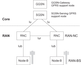
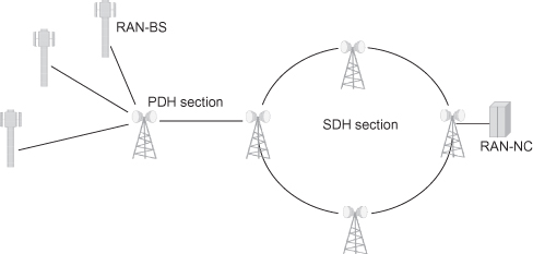
Backhaul networks employ a range of different technologies designed in a variety of architectures and use a wide set of terminology and jargon. In this chapter, we will refer to mobile backhaul as the radio access network (RAN) between a cellular base station at the cell site and the network controller site or the edge core node. We will use the terms RAN-BS and RAN-NC as defined by the Metro Ethernet Forum (MEF) Mobile Backhaul Implementation Agreement (MBH-IA [19]). RAN-BS, the RAN Base Station, stands for any mobile technology base station such as GSM, CDMA, or Wimax base stations (BTS), a 3G Node-B, or LTE eNB (evolved Node-B). RAN-NC, the RAN network controller, stands for GSM base station controller (BSC), 3G RNC, Wimax access service network (ASN) gateway, or LTE serving gateway (SGW).
As an example, Figure 6.5 describes 3G architecture; the mobile backhaul in this case includes primarily the interface called “Iub” between node-B’s and RNC, and the interface called “Iur” between RNCs. The first part of the RAN connecting the RAN-BSs is often referred to as the access RAN, whereas the part connecting the RAN-NCs is referred to as the aggregation RAN. The access RAN may include thousands of base station connections typically aggregated over several steps. Therefore the emphasis in access RAN systems is on efficiency and low cost. The aggregation RAN, on the other hand, is more limited in scale, but with much more strict resiliency requirements.
Figure 6.5. 3G architecture.
Mobile backhaul networks have traditionally been realized using TDM and ATM technologies. These technologies are transported over the PDH radios in the access RAN, and SDH/SONET radios in the aggregation RAN.
Next-generation mobile equipment and networks, however, will be based on Ethernet. Carrier Ethernet services will provide the connectivity in the mobile backhaul network, either in dedicated Ethernet networks or in a converged network together with fixed services. We will examine the technical aspects of microwave radios both in legacy networks and in Ethernet networks, and examine the evolution paths from legacy to next-generation radio networks.
6.4.2 PDH and SDH Radios
The most common legacy interfaces in mobile access backhaul are E1 and T1 used to multiplex a number of 64-Kbps voice PCM channels (32 at E1, 24 at T1), and they became the common interface for legacy 2G GSM and CDMA base stations. Newer technologies, such as 3G UMTS, use ATM over the same TDM E1 interfaces or over a bundle of such interfaces [referred to as IMA (inverse multiplexing)], and CDMA2000 uses HDLC over T1s or DS-3.
Legacy mobile backhaul networks are typically deployed in either a tree or a ring topology, or a combination of these, as shown in Figure 6.6. The backhaul network collects multiple E1/T1s from the cell sites and transports them toward the core. Tree topologies require low-capacity links at the access edge, and they gradually increase capacity requirements as the network advances toward the core. PDH radios offering bandwidth in increments of either E1 (2 Mbit/s) or T1 (1.55 Mbit/s) are widely used in such deployments. Ranging from low-capacity/low-cost 4xE1/T1s radio links at the tail site (the last base station in a network) PDH radios can reach 64xE1/T1 or more connections at higher aggregation levels.
Figure 6.6. Legacy PDH/SDH backhaul example.
At the aggregation RAN, connections have higher capacity and resiliency is more important, and thus SDH/SONET radios are often used. Such radios were developed to replace the PDH system for transporting larger amounts of traffic without synchronization problems and with supported resiliency over ring deployments. Since the RAN-NCs connect several hundreds of cell sites, often its interface is STM-1/OC-3, which supports 155 Mbit/s of throughput; and the aggregating rings, built of fiber optics or microwave SDH/SONET radios, can be of multiple STM-1, STM-4, or even more. Modern SDH radios support bandwidth in increments of STM-1, up to 2xSTM-1 over single carrier, or 4xSTM-1 with dual carrier (possibly over same channel using XPIC).
An E1/T1 path from the RAN-NC to the individual cell site may consist of many “hops” across the metro ring and over the access tree. To ensure ongoing and uninterrupted communication, the radio system must maintain the signal performance parameters over this multihop path. A radio delivering TDM signals should not only reconstruct the E1/T1 data at its remote side, but also perform two major requirements: fault management and clock delivery.
TDM signals use fault management indications such as AIS (alarm indication signal) and RDI (remote defect indication) that are propagated in responses to signal loss or signal out of frame. AIS and RDI serve to alert the rest of the network when a problem is detected. A TDM radio should initiate such indications at its line ports, also in response to radio link failures.
Clocking performance is a major issue for some legacy base stations that use the TDM signals not only for delivering traffic but also for synchronization. Degraded synchronization may result in poor performance of the cellular network, and the critical handover procedure in particular. The ITU G.823/G.824 [7,8] standards define two kinds of TDM interfaces: traffic interface and synchronization interface. Each has its requirements for short-term phase variations, referred to as jitter, and long-term phase variation, referred to as wander (defined as slow phase variations, at a rate of less than 10 Hz). Note that some base stations (such as CDMA) use external synchronization signals (usually GPS). In these cases, TDM synchronization over the radio network is not an issue.
A radio link that delivers TDM signals must maintain the clock for each delivered signal over the radio link. Since typically the radio itself uses an independent clock for transmission which is not related to the line clock, it utilizes justification bits to align the clocks at the transmit side. This technique also restores the line clock at the receive side using a clock unit. In the case of PDH, this is performed separately for each E1/T1 signal.
It is important to note that clock performance is degraded as the number of radio hops between two end points increases. Hence, there is a limit to the number of radio hops that can be supported without aligning back to a common clock from a reliable external source.
Cross-Connecting.
Traditional radio network implementations used PDH radios for transport and connected them to each other using a manual wiring device called a digital distribution frame (DDF). Modern radio systems may already include a multiradio platform with embedded cross-connect function. This provides a one-box solution for radio aggregation sites and adds advantages such as better reliability, improved maintenance with a common platform to manage, and the ability of remote provisioning. Not the least bit important, a single-box solution makes for smaller system footprint and will most likely have a better cost position.
In aggregation sites closer to the core, a large quantity of signals is connected, and it becomes cumbersome to use separate connections for each E1/T1. Hence radio systems with cross-connect are usually groomed for capacity interfaces such as channelized STM-1.
Resiliency.
Resiliency is another important aspect in radio network deployment. Resiliency ensures the network’s reliability and overall service quality and should be treated at the element level and the network level. Radio networks need to be resilient from both equipment failures as well we from radio link failure due to propagation effects as heavy rain fade. Resiliency is an important consideration when designing the network’s topology. In a network built in a tree or chain topology, the closer a failure is to the core, the more cell sites it can put out of service; therefore operators typically employ protected radio links in aggregation sites where a single link failure can affect a significant portion of the network. Such an example is depicted in Figure 6.7a below where each radio link affecting more than one cell site is protected. It is important to note that this protection scheme shields against equipment failures, but not against propagation effects that will influence both radios in a protection scheme, nor against a complete site disaster.
Figure 6.7. Backhaul resiliency. (a) Protected links in a tree backhaul. (b) Resiliency in a ring backhaul. (c) SNCP resiliency in a general (mesh) backhaul.
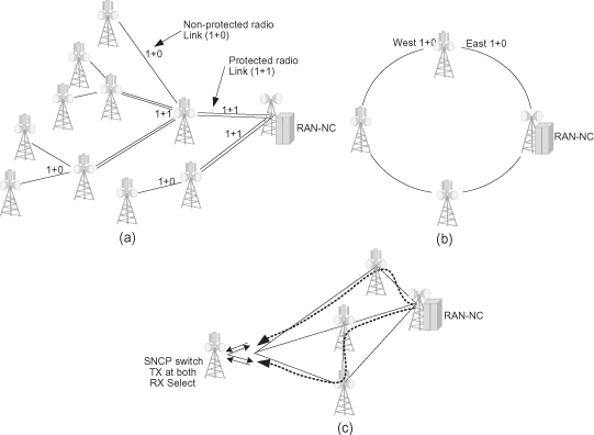
In ring deployments, resiliency is inherent in the topology because traffic can reach each and every node from both directions, as shown in Figure 6.7b. Thus, there is no need to protect the radio links, so typical ring nodes feature unprotected radio links in both east and west directions. One additional advantage that rings have over tree topologies is that ring protection not only covers equipment failures, but also provides radio path diversity that can help in dealing with propagation fading.
SONET/SDH rings offer standardized resiliency at the path level and can be deployed in several architectures, such as UPSR or BLSR [9]. When deploying PDH rings, path protection may be handled over the entire ring (similar to SDH but proprietary because there is no available standard) or on a connection-by-connection basis, providing end-to-end trail protection using subnetwork connection protection (SNCP). The common way to implement SNCP would be 1 + 1, which means that traffic is routed over two diverse paths, and a selector at the egress point selects the best path of the two. SNCP can be used in other topologies as well. Figure 6.7c depicts an SNCP implementation for a partial mesh case. The SNCP can be defined at different levels and is usually applied at the E1/T1 level.
6.4.3 Ethernet Radio
Types of Ethernet Radio.
Ethernet radio can be described as an Ethernet bridge in which one (or more) of its ports is not an Ethernet physical layer (PHY), but a radio link. The unique characteristics of the radio introduce a certain level of complexity and therefore require special planning of the bridge.
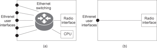
Simple radios typically feature two ports: a line port and a radio port (Figure 6.8). Such systems are sometimes referred to simply as “pipe,” since traffic flows only from the line to the radio and vice versa. Yet, even such “simple” systems have a certain level of sophistication which varies from basic “transparent” devices that feature no traffic processing, to sophisticated two-port devices, capable of a variety of classifications and VLAN encapsulations, bridging for inband management and sophisticated traffic management along with features such as policing and shaping, OA&M support, and more.
Figure 6.8. Types of Ethernet radios. (a) Multiport switched Ethernet radio. (b) “Pipe” Ethernet radio.
Some very basic radios, for example, are designed to directly modulate the carrier with the physical Ethernet signal. Such radios would deliver even faulty signals, with error frames, since they lack an Ethernet MAC function. Other radios may include Ethernet MAC and drop errored checksum frames. In order to allow radio inband management, a bridging capability is needed to bridge the management frames to the CPU and vice versa (usually tagged by a unique defined management VLAN).
Multiport devices, on the other hand, may include several line ports and several radio ports to provide an integrated radio node solution. Such systems also vary from very basic systems such as “multipipes” lacking bridging functionality between ports, to full-blown sophisticated bridges.
Framing.
Native packet radios differ from legacy PDH/SDH radios in that traffic is delivered in bursts and in different-sized frames rather than a continuous fixed rate of traffic. On the other hand, the radio link still delivers a continuous bit rate that may be either fixed or dynamic with ACM. In order to carry frames on such a continuous transmission, the radio system marks the beginning of each packet and also fills in the “silent” gaps between frames. Common techniques for this task are HDLC (High-Level Data Link Control) and GFP (Generic Framing Protocol) defined by the ITU-T to allow mapping of variable-length signals over a transport network such as SDH/SONET.
Rate Gap Between Line and Radio.
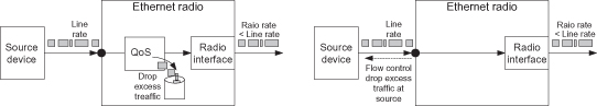
A challenging issue of packet radio is line rate and radio rate differences. One of Ethernet’s greatest advantages is its scalability. A fast Ethernet (FE) line can deliver every rate up to 100 Mbit/s, while a gigabit Ethernet (GbE) line can deliver up to 1000 Mbit/s.1 A GbE radio will usually not support the full line rate, creating a congestion problem. Congestion happens not only when the average bit rate of the radio line exceeds the radio link rate, but also when long bursts occur in the line.
Let us consider the following example: a GbE interface supports an average traffic rate of 200 Mbit/s and utilizes a radio link of 200 Mbit/s. Since each frame enters at the line rate of 1 Gbit/s and is transmitted at 200 Mbit/s, it takes five times longer to egress than ingress, thus requiring a buffer to hold the burst of data until it is transmitted. As long as the bursts are not bigger than the buffer size, no congestion will occur. But take, for example, an entire minute of full GbE traffic followed by 4 minutes of silence, which is still 200 Mbit/s of traffic on average. In this case, the burst size is much bigger than any practical buffer, making traffic loss unavoidable.
A radio system can handle congestions in one of the following two alternatives, as depicted in Figure 6.9: Drop the excess traffic frames in the radio, or avoid any excess traffic in the radio by signaling backwards to the source so it can drop it (also known as flow control). Dropping frames in a way that least affects the end-to-end service requires a Quality of Service (QoS) mechanism with buffers large enough to accommodate the desired burst size. Large buffers obviously increase latency and cause a problem to real-time services. Still, good QoS planning can solve such issues by classifying the traffic into different classes, allowing real-time delay-sensitive flows (such as voice and video calls) to receive higher priority with small buffering, whereas non-real-time traffic (as web browsing or files transfer) will be classified to lower priority with larger buffering.
Figure 6.9. Handling the rate difference between line and radio.
It should be noted that the majority of data traffic today consists of “elastic flows” such as TCP-IP or FTP which are non-real time and not delay-sensitive. Only small portions are actually “streaming flows” like voice or real-time video which are delay-sensitive and require a constant bit rate.
The second option for handling the difference between line rate and radio rate is to signal back to the feeder in case of congestion. The common mechanism for doing so is by employing Ethernet flow control (802.3x). This mechanism, however, has a number of drawbacks. First, it stops all the data without any consideration to priority. Second it can introduce latency that may lead to packet loss if no sufficient buffering exists. This may happen because flow control messages are carried “inband” as Ethernet frames and as such may be delayed behind other large data frames. In such case, buffers may reach congestion before the flow control message reaches the feeder. Lastly, careless use of flow control can spread the back pressure in the network and turn a local problem into network-wide one.
Ethernet Radio QoS.
As mentioned, QoS is a key performance issue in Ethernet radio due to the difference between (a) consists line rate and radio rate and (b) the varying rate of ACM radio. A basic Ethernet QoS mechanism is of (a) a classifier that sorts the traffic frames into different priority queues and (b) a scheduler that selects the order at which traffic frames are transmitted from the queues
Simple classifications can be based on different markings such as the Ethernet frame VLAN ID, VLAN priority bits (the 802.1p standard defines 8 classes of service) or the layer 3 (IP) priority bits marking (such as IPv4 TOS/DSCP that defines 64 classes of service). MPLS EXP bits may also be used in the case of IP/MPLS carried over Ethernet. Such classifications will typically use 4 or 8 queues, whereas more sophisticated classifications can be based on traffic flows and utilize a much larger number of queues.
Common scheduling methods are Strict Priority (SP), Weighted Round Robin (WRR), Weighted Fair Queuing (WFQ), or a combination of these. Assigning a queue to higher SP means that as long as there is even a single frame in this queue, it will be transmitted first. In case other queues are overloaded at this time, frames of lower SP queues will be discarded.
Unlike SP, WRR and WFQ select frames from all non-empty queues according to assigned weights. Often a combination of the methods is used, for example to give strict priority to extremely important traffic such as synchronization where other queues are scheduled using WRR.
Bandwidth management and congestion avoidance are two additional mechanisms that are commonly used for Ethernet QoS. The bandwidth management mechanism includes rate limiters (policers) and traffic shapers. These may be implemented at the port level and at the queue level, as well as per VLAN tag or per traffic type such as unicast/broadcast. For example, introducing a policer at each queue allows enforcing a bandwidth profile per class of service. Introducing an egress shaper allows the conformation of the egress rate of the line (or radio) and smoothes traffic bursts to better utilize its bandwidth.
Congestion avoidance mechanisms include such algorithms as Random Early Detection (RED) and Weighted RED (WRED). These mechanisms aim to improve the performance of TCP flows in the network by early discarding frames already before the queue is congested. The random dropping eliminates the process known as TCP synchronization, where multiple TCP flows are simultaneously slowing, resulting in an underutilized network.
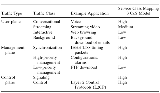
Class of Service (CoS) Levels.
For effective QoS operation, one should define the network service classes. As an example, Table 6.3 describes the 3GPP definition for traffic classes and their mapping into the mobile backhaul network service classes. The example uses the 3 CoS model, which is one of the models defined by the MEF CoS IA (draft). The model uses three classes: high, medium, and low. Each level is associated with its identifier (such as VLAN tag priority bits or IPv4 DSCP) and has performance attributes such as bandwidth, frame loss, frame delay, and frame delay variation. Other models can map the same traffic types into other CoS levels.
TABLE 6.3. 3GPP Traffic Classes and Mapping to 3 CoS Model
Ethernet Adaptive Modulation (ACM) Radio.
One of the advantages Ethernet radio has over PDH/SDH radios is the ability to transport only part of the data using ACM, without dropping all of it when propagation conditions do not allow the radio to work at its maximum capacity. In order to handle the reduced bandwidth, QoS must be implemented, so that frames are not dropped randomly but rather in order of importance, according to the operator service policy.
ACM radios have another advantage when delivering TCP/IP data. In a non-ACM radio, even a short interruption of 50 ms can cause TCP/IP timeouts. As a result, drastic throughput decrease can occur until the TCP sessions are recovered, a process that may even take as long as several seconds. With ACM radio, complete traffic interruption is avoided, but instead there is only a momentary drop in throughput. This is not likely to cause any TCP timeouts, and the TCP flow can handle any loss by adjusting and dropping the rate.
One Ethernet transport aspect that is intensified by ACM is delay variation. As ACM radio rate drops to lower rate, it introduces more latency. Thus delay variation is worse with ACM than it is with fixed modulation. This introduces challenges in some applications, such as synchronization over packet, as will be explained further in this chapter.
Ethernet Radio Optimizations.
The Ethernet physical layers defined by the IEEE 802.1 standard, uses some non-payload fields such as Preamble and Start Frame Delimiter (SFD), as well as Inter frame Gap (IFG) following each frame. These fields are not required by the radio media and can be easily reconstructed at the far-end radio, saving up to 25% of the bandwidth with short frame length.
Further bandwidth savings can be achieved by omitting the CRC and recomputing it at the far end. In order to avoid fault frames, there is a need to monitor radio performance and drop radio payload frames in case of errors. Thus this may have penalty of error multiplication, as radio code words are not synchronized to the Ethernet frames, and one errored word can cause the drop of several frames even in cases where not all of them were indeed errored.
More sophisticated optimizations techniques include compressions, such as MAC header compression, or even higher layers header compression (IP, UDP, TCP, etc). Since such headers may repeat themselves many times during a stream of traffic, it is possible to deliver a frequent “headers map” to the remote side and then transmit a short ID instead of the long header. The saving in such a case is dependent on the nature of traffic. If traffic actually turns out to be random, there may be even a loss of bandwidth resulting from transmitting the key maps. In many mobile applications, a limited number of connections may exist so such optimizations can yield a significant saving (results up to 25% were demonstrated by leading vendors).
Compression at higher layers and payload compression should be carefully considered according to traffic nature, since it can bring benefit, but also may become useless. For example, IP header compression (as defined by IETF RFC 2507/2508/3095) may be useless in UMTS networks, since 3G already employs it in itself. Payload compression may also be useless if encryption is used in the network, due to the random nature of encrypted data.
Carrier Ethernet Radio.
Traditional Ethernet LAN is based on frames forwarding according to dynamic learning tables, as well as on frames broadcasting in case the target address is unknown. Such networks are also based on Spanning Tree Protocols (STP) for preventing loops in the network. When deploying carrier networks, the use of learning and STP yields poor performance; it is not scalable and does not utilize the network resources in an efficient way, nor does it allow traffic engineering or fast resiliency.
The MEF, under the mission of accelerating the worldwide adoption of carrier-class Ethernet networks and services, sets the requirements and attributes that distinguish carrier Ethernet from familiar LAN-based Ethernet. These include primarily a definition of standardized services and requirements of QoS, reliability, scalability, and service management.
The defined services include a few types of Ethernet connections (EVC) [18]: a point-to-point Ethernet connection called E-line, a multipoint-to-multipoint connection called E-LAN, and a rooted point-to-multipoint connection called E-tree. Reliability means demanding availability and rapid (sub-50 ms) recovery time. QoS, setting, and provisioning service level agreements (SLAs) that deliver end-to-end performance based on bandwidth profile, frame loss, delay, and delay variation are additional requirements. Service management requires carrier-class OAM and an ability to monitor diagnose and manage the network.
Carriers evolving to Ethernet backhaul are not likely to rely on LAN-based Ethernet, but rather demand tools to engineer the traffic and to provision and manage connections with defined SLAs. In the following sections we will describe some aspects of carrier Ethernet required in today’s modern radios for carrier applications as mobile backhaul.
It should be noted that different technologies can be utilized to implement these capabilities over Ethernet, from simple (and limited scale) VLAN tagging (802.1Q) [17], to provider-bridging (802.1ad), provider backbone bridges (PBB—802.1ah) [22], provider backbone bridge traffic engineering (PBB-TE) [23], and VPLS/VPWS over MPLS (multiprotocol label switching)-based technologies. The MEF does not define the “how” but rather the “what.” The right choice of technology depends on many variables. While at the fiber core of the networks MPLS is the dominant solution, for more limited-scale segments of the network including mobile backhaul, simpler solutions can suit better. This is true in particular when it comes to radio networks in which bandwidth is not unlimited, and the overhead introduced by more sophisticated technologies can be a burden.
OAM (Operations, Administration, and Maintenance).
OAM refers to tools needed to detect and isolate faults, as well as to monitor the performance of the network connection. Such tools are a crucial requirement in any carrier network because they enable the detection of link failures, verification of end-to-end connectivity, and monitoring the network’s performance.
Originally, Ethernet had no OAM tools; however, in recent years, new standards were introduced to address the need for Ethernet OAM over carrier and service provider network. Such standards include: IEEE 802.3ah (Ethernet in the First Mile), which deals with link level monitoring; IEEE 802.1ag [16] (and also ITU Y1731), which deals end-to-end service connectivity fault management (CFM); and ITU Y1731 [15], which, in addition to 802.1ag CFM, also defines Ethernet performance monitoring (PM).
Ethernet OAM defines monitoring points known as maintenance end points (MEPs) and maintenance intermediate points (MIPs). MEPs are located at the edge of the Ethernet service, at the user–network interface (UNI), or at the network-to-network interface (NNI), where MIPs are located within the Ethernet network at intermediate points of the connection. MEPs can generate various OAM test frames in the Ethernet data stream and respond to OAM requests, whereas MIPs can only respond to OAM requests.
The basic CFM operation of a MEP is to send periodic connectivity check messages (CCMs) to other MEPs belonging to the same service. In a normal operation, each MEP periodically receives such messages from all other MEPs. If CCMs fail to arrive, the MEP detects that a failure occurred in the connection. MIPs are used in the process of fault isolation, responding to loopback requests (similar to IP ping) or link-trace requests used to trace the path of the service. Ethernet OAM defines eight maintenance levels of operation to allow seamless interworking between network operators, service providers, and customers.
For the Ethernet radio being part of carrier Ethernet networks, implementing OAM is a crucial requirement, as is the case for any other bridge in the network.
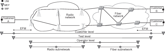
Figure 6.10 shows an example of a network connection between three customer sites, across two networks. Both the operators and the customer are using OAM to monitor the connection by locating MEPs and MIPS along the connection, each at different maintenance levels. In addition, EFM is used at both connections to monitor the line link between operator and customer.
Figure 6.10. Ethernet OAM.
Resiliency.
As Ethernet evolves to carrier networks, resiliency requirements become just as important as it is for legacy TDM networks. As with OAM, originally Ethernet had no such tools, but new standards were developed to provide rapid service restoration that deliver SDH/SONET grade resiliency. These include (a) ITU-T G.8031 [14] for Ethernet linear protection switching and (b) G.8032 [13] for Ethernet ring protection switching (ERPS). The objective of fast protection switching is achieved by integrating Ethernet functions and a simple automatic protection switching (APS) protocol.
When considering tree or chain topologies in which path redundancy cannot be found, Ethernet networks employ the same methodology as presented in the TDM case; that is, radio protection handles equipment failures. It is important to mention in this respect the use of a link aggregation group (LAG) in order to connect protected equipments. When a logical link consists of a LAG and one or more members of the LAG fails, the LAG continues to deliver traffic with reduced capacity; thus LAG is a simple common way to connect the protected radio to the fiber switch feeding the wireless network.
When considering a general (mesh) topology network, spanning tree protocols (STP) are often used. However, since convergence time is very long, typically >30 s for STP and 1 s for rapid STP (RSTP), it is not suitable for carrier networks where 50 ms is the industry benchmark traditionally achieved by SONET/SDH.
Ring STP and G.8032 ERPS.
Though not standardized, many vendors have created ring-optimized enhancements of RSTP, allowing fast restoration that approaches the 50-ms goal. STP uses bridge protocol data units (BPDUs) that propagate in the network and need to be processed at every node with complex tree computation. The ring STP takes advantage of the known and simple topology of the ring, whereas the tree computing simply results in the selection of one port to be blocked. Thus it is able to process and propagate the BPDUs much faster and achieve the required fast convergence time.
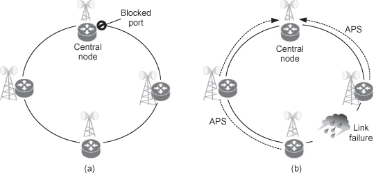
A similar approach is taken by the recent ITU-T standard protocol G.8032, which is designed to achieve sub-50-ms ring resiliency in a ring topology. Also dubbed ERP (Ethernet ring protection), G.8032 defines a central node that blocks one of its ports, thereby blocking one link in the ring and not allowing a loop to be formed for the Ethernet traffic. OAM CCMs are then used to detect a link failure in the ring, while automatic protection switching messages (APS) are used to announce such a failure and trigger the opening of the blocked link, as shown in Figure 6.11. For sub-50-ms protection, fast CCM rate of 3.3 or 10 ms is needed.
Figure 6.11. Ethernet ring protection. (a) Initial ring state (central node blocks one port). (b) After a link failure (blocked port is now open).
For Ethernet radios in a ring, the implementation of ring STP or ERPS is a key issue in supporting carrier ethernet service. The implementation should not differ from any wire-line device, but rather it has to be able to initiate an APS request when radio failure events occur.
G.8031 Ethernet Linear Protection Switching.
As mentioned, a carrier Ethernet network will not likely be based on LAN Ethernet concepts (learning and STP), but rather it will based on an engineered connection. With general mesh networks, it is possible to define more than one path for E-line EVC and have a redundant path protection. Just as SNCP described for protecting TDM trails, G.8031 specifies point-to-point connection protection schemes for subnetworks constructed from point-to-point Ethernet VLANs.
Protection switching will occur based on the detection of certain defects on the transport entities within the protected domain, based on OAM CCMs and using APS protocol. For sub-50-ms protection, a fast CCM rate of 3.3 or 10 ms is required.
G.8031 defines linear 1 + 1 and 1 : 1 protection switching architectures with unidirectional and bidirectional switching. Using 1 : 1 has the benefit of utilizing the standby path bandwidth as long as it is not active (but just running CCMs), whereas 1 + 1 consumes both paths bandwidth constantly. In this respect we can highlight the benefit of Ethernet over TDM trails with SNCP, where the standby path bandwidth cannot be used by other services because there is no statistical multiplexing.
G.8031can fit any general topology; it allows utilizing the network in an optimal way by engineering the connections in the optimal working path and diverse path.
6.4.4 The Hybrid Microwave Radio
The hybrid radio combines both TDM traffic and Ethernet frames simultaneously while keeping the important characteristics of both. It has the capability of keeping the TDM clock attributes and allowing it as traffic and synchronization interface, as well as the capability to transport the Ethernet frames natively and being able to drop frames under ACM conditions according to QoS policy. The radio bandwidth can be dynamically allocated between the TDM fixed bandwidth and variable Ethernet bandwidth to optimally combine both kinds of traffic. Unused E1/T1 bandwidth should be automatically allocated for additional Ethernet traffic.
In early deployments, in which Ethernet is primarily added for lower-priority “best-effort” data services, it is assumed that under fading situation with ACM, the hybrid radio will first drop only Ethernet traffic and then keep the TDM voice and real-time traffic connections. With network convergence and new deployments of Ethernet-based services, this does not always have to be true. Thus, more sophisticated solutions should be configured to drop some lower-priority Ethernet traffic first, but also allow the higher-priority Ethernet to be the last to drop—even after lower-class TDM connections have been.
6.5 MOBILE BACKHAUL EVOLUTION ALTERNATIVES
The evolution from 2G to 3G to LTE and onwards goes hand in hand with the shift from voice (2G) to data (3G) and to fully mobile broadband connectivity (LTE/4G), together with the shift from circuit to packet connectivity. Another migration is the one toward convergence of fixed and mobile networks, in which the same backhaul network serves not only the mobile network but also that of fixed services such as business or residential broadband access and VPNs.
The growing demand for mobile data services requires enormous capacity growth in the backhaul segment, which makes TDM backhaul neither scalable nor affordable anymore. For example, LTE eNB backhaul requires 50xE1s (supporting 100 Mbit/s), compared to 2xE1s used at typical 2G BTS. When multiplying this number by the number of cell sites in a network, it’s plain to see that simply adding E1 connections makes no sense.
In addition, the latest mobile technologies introduced like WCDMA-R5 and onwards—EVDO, LTE and WiMAX—are “All-IP” technologies and are based on pure packet architecture. This makes Ethernet the natural first choice for backhaul growth.
Up to this point, we have counted a number of advantages that Ethernet has over TDM. But in order for Ethernet to completely displace TDM, it must provide the necessary carrier Ethernet requirements of QoS and OAM. Additionally, next-generation Ethernet systems must ensure synchronization delivery and fast resiliency while supporting legacy TDM. Though Greenfield and long-term deployments may be Ethernet only, existing legacy networks will not quickly disappear, but will continue to coexist with new technologies for many years to come.
6.5.1 The Migration: Evolving to Ethernet While Supporting Legacy TDM
Figure 6.12 depicts the evolution of mobile networks and backhaul technology. For each technology, the diagram indicates the maximal user throughput, and describes a typical RAN-BS deployment case. In the following sections we will discuss three different alternatives for backhauling next-generation mobile traffic over radio networks:
1. Pure TDM backhaul
2. Pure packet backhaul
3. Hybrid backhaul, with overlay of both networks
Figure 6.12. Mobile networks evolution.
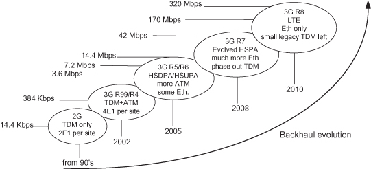
TDM, hybrid, and all-IP backhaul can be served by copper, fiber, and radio transport systems. Each alternative has its strong and weak points, and there is no single “right way.” In the long run, telecom operators hope to implement all-IP 4G architectures for reasons of simplicity and cost-cutting. However, until reaching maturity of pure packet backhaul and considering the fact that 3G and even 2G networks will not disappear overnight, we can assume that all of these alternatives will coexist together for a long time.
6.5.2 Pure TDM Backhaul
Keeping the legacy TDM (PDH/SDH) network in the long term is a valid option; but over time, legacy technology will be outmatched by the advancement of mobile technologies. While HSDPA initial deployments still used TDM interfaces and required only few additional E1/T1s to carry data services, next-generation cellular base stations are expected to have Ethernet interfaces and fit into all-IP architectures.
Mapping Ethernet frames over TDM is not a new concept, but operators who chose this solution will quickly run into scalability and performance issues. Maintaining RANs based on costly E1/T1 connections to support data rates in the tens or even hundreds of Mbps per cell site is not likely to generate a profitable business case.
While this book is being written, some microwave radios still do not support native packet transport. Such systems implement Ethernet transport by mapping frames on groups of E1/T1 connections that are carried all over the network as fixed-rate circuits. This solution obviously has several drawbacks including: granularity, as bandwidth is allocated at multiples of E1/T1; scalability, as a very large number of E1/T1s are gathered along the network; and, most important, no statistical multiplexing is available at the network’s aggregation points. An exception for this is the use of ATM aggregation which allows statistical multiplexing for ATM-based traffic as with 3G early releases, yet this option is not future-proofed for IP-based technologies.
6.5.3 Packet-Only Backhaul
A pure packet backhaul appeals primarily as it is future-proofed and provides the complete solution over a single technology. As such, it has the potential of saving in both CAPEX and OPEX, but also maintains some risks and drawbacks.
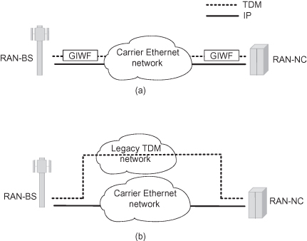
A pure packet backhaul requires us to map the TDM/ATM traffic over packet using TDM to Packet Generic Inter-Working Function (GIWF), as shown in Figure 6.13a, in contrast to maintaining the legacy network in the hybrid backhaul concept shown in Figure 6.13b.
Figure 6.13. Hybrid backhaul and pure packet backhaul. (a) Pure packet backhauling. (b) Hybird backhaul concept.
Several standards define the emulation of TDM/ATM over a packet-switched network (PSN). These include IETF pseudo-wires (PW) [24,25], MEF circuit emulation services over Ethernet (MEF8) [20,21] and some ITU-T recommendations. The IETF long list of RFCs and ITU-T recommendations define PWs for most traditional services as TDM, ATM, frame relay, Ethernet, and others. Thus it allows the use of a single-packet infrastructure for all. The major benefit of using emulated solutions is the ability to map everything over the same network and thus install, manage, and maintain a single network for all service types. A major drawback is the overhead introduced by the encapsulation of frames. While such overhead may be insignificant at the fiber core, it can become a major problem over copper and microwave in the access and metro. The encapsulation overhead depends on the exact configuration and can be reduced by using larger frames that encapsulate more TDM/ATM traffic at a time. Yet this approach results in longer delays and error multiplication.
It should be noted that at some implementations, such as IP/MPLS PW, the overhead will be introduced not only to the TDM traffic, but also to the Ethernet traffic, as several PWs are assigned to all types of traffic coming from the cell site. Thus in such implementations, Ethernet packets are encapsulated by IP/MPLS PW headers, and then transported again over Ethernet, resulting in a significant bandwidth overhead and low radio utilization.
Another major issue with pure packet backhaul is delivering synchronization over the packet network while meeting the requirement for TDM services (G.823/G.824) [7,8] under many network conditions. Synchronization between RAN-BSs is critical to the mobile network performance. A requirement of ±50-ppb clock accuracy is defined for GSM, 3G, and LTE FDD systems, and systems need to comply with strict jitter and wander specifications. With the exception of a few networks that utilize an external source for the clock delivery (usually a GPS receiver, which is commonly used in IS-95/CDMA2000 networks), most legacy networks use SDH/PDH backhaul to deliver synchronization.
As shown in Figure 6.14a, the TDM generated in a central site (MSC) is locked to a primary reference clock (PRC) via a synchronization interface (such as E1 or STM-N). The RAN-BS is synchronized on the backhaul incoming TDM traffic signal, so eventually it locks the RAN-BS to the same PRC. When using PW/CES backhaul, the RAN-BS is now synchronized on the TDM recovered from CES frames.
Figure 6.14. RAN-BS synchronization methods at the backhaul. (a) TDM synchronization. (b) Timing over packet synchronization. (c) Synchronous Ethernet synchronization.
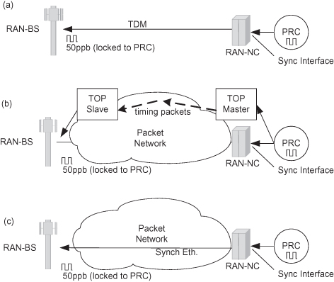
Standards that define the delivery of timing over packet (TOP) are IEEE Precision Time Protocol (PTP) 1588v2 and IETF NTP. Both are based on exchanging time information via dedicated timing packets (using time-stamps) and restoring the clock using this information, as shown in Figure 6.14b. Such techniques are ubiquitous and work over any transport technology, but the restored clock accuracy is highly dependent on the network performance in terms of packet delay variation (PDV). Whatever sophisticated algorithms are employed at the clock restoration, there are limits to the accuracy that can be achieved as the PDV gets too high.
When observing the Ethernet backhaul network, PDV becomes more of an issue as the radio links are narrower in bandwidth. We can observe a simple test case of a cell site with a backhaul connection of 5 Mbit/s versus a 50-Mbit/s radio link. At the cell site, TOP frames are transmitted at a fixed rate, but also large data frames of 1500B may be transmitted in between. Obviously the TOP frames should be classified to higher-priority queue and scheduled with strict priority, but it may happen that such a frame is scheduled just after a large data frame (known as “head-of-line blocking”) and delayed longer. Since the transmission time of a 1500B frame is only ∼0.24 ms at the 50-Mbit/s link versus ∼2.4 ms at the 5-Mbit/s link, the PDV will be 10 times higher at the narrow bandwidth link. To calculate the total end-to-end PDV, one should consider several connection hops. Still, because usually the closer we are to the core, the larger the connection’s bandwidth becomes, the dominant contributor to PDV is the access network.
There are proprietary methods to mitigate the problems discussed above in a radio link; however, it is important to keep it mind that with standard Ethernet transport, time over packet is risky when it comes to access networks, because it is highly dependent on PDV performance.
A different technique to deliver synchronization over Ethernet backhaul is synchronous Ethernet (ITU-T G.8261) [10], shown at Figure 6.14c. Synchronous Ethernet, or Sync-Eth, is a physical layer frequency distribution mechanism similar to SDH/PDH that uses the actual Ethernet bit stream to deliver the clock. Its biggest advantage is that the clock accuracy is independent from network load. Additionally, it has no demands on bandwidth resources and is not affected by any congestion or PDV. Thus Sync-Eth represents an excellent SDH/PDH replacement option.
Sync-Eth drawbacks are that it requires special hardware at every node, it is limited to a single clock domain, and, unlike ToP, it can only deliver frequency and not phase.
A radio supporting Sync-Eth should have the capability to deliver the output Ethernet traffic at the remote side, locked to input clock at the near side and maintaining its quality (jitter and wander as specified by G.823/G.824). As PtP radio naturally delivers the clock of the transmitted signal, supporting Sync-Eth is relatively easy. Additional functionality is required to (a) select timing from several inputs for network protection and (b) provide timing traceability via SSM (Synchronous Status Messages).
6.5.4 Hybrid Backhaul
Hybrid backhaul means overlaying existing circuit backhaul networks with a carrier Ethernet transport layer used for data traffic and for connecting base stations with IP interfaces, as shown in Figure 6.13b. This solution allows keeping the legacy connections and synchronization over TDM, while adding flexibility, increasing capacity and enjoying additional benefits using a packet network.
The concept of hybrid is sometimes referred to in the wireline backhaul segment as “offload.” In the wireline world, hybrid systems sometimes use a different media for each kind of network—for example, maintaining the TDM over leased lines and delivering Ethernet over DSL. This method has an upside of more cost-effective delivery of data using DSL and has the obvious downside of having to manage and maintain two separate networks. In the wireless world, hybrid means having two logical networks on a single physical network. Figure 6.15 demonstrates a hybrid aggregation network, where each tail site is accessed with both Ethernet and several E1/T1 interfaces. Each aggregation site includes a node with TDM cross-connect and an Ethernet switch. All traffic is gathered finally toward the core: Ethernet on a GE interface, and all TDM on a channelized STM-1 interface.
Figure 6.15. Hybrid radio backhaul network example.
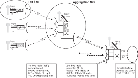
Enabling smooth migration of the backhaul is a complicated task. Still, in many cases the hybrid approach, employing radios with ACM, carries the lowest risk. Figure 6.16 shows a typical migration case for legacy TDM network based on microwave radios carrying 4xE1s per site over 7 MHz or 14 MHz channels. Adding the new Ethernet traffic for data services is possible while maintaining the same radio planning and antennas. Enabled data rates are up to 50 Mbit/s over 7 MHz channels or 100 Mbit/s over 14 MHz channels, while the TDM traffic stays the same, thus without any synchronization issues.
Figure 6.16. Migration of RAN-BS connection from TDM to hybrid.
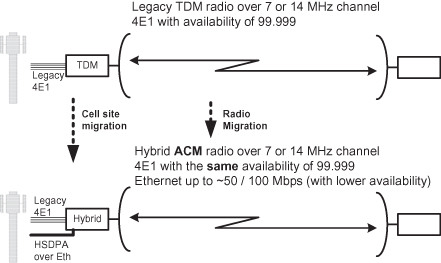
We can see the importance of ACM, being the enabler for such migration. Without ACM, legacy services could not be maintained with the same service level; thus radio planning would have needed to redesign (such as using bigger antennas), and migration cost would have been significantly higher.
6.5.5 Hybrid Access with Packet Aggregation
We mentioned the difficulties and risks of pure packet backhaul, especially when it comes to the access portion, where there is narrower available bandwidth. In the access segment the PDV is higher, and the overhead of solutions like PW is more significant. On the other hand, a pure packet backhaul has its advantage of convergence and simplicity, managing all kinds of traffic over the same network.
A solution that combines a hybrid access network and pure packet with PWs at the aggregation network can benefit from all advantages and avoid some risks. It also has the potential of cost saving as PW equipment is not needed at every site, but only at the aggregation sites, as depicted in Figure 6.17.
Figure 6.17. Combining the hybrid and the packet backhaul.
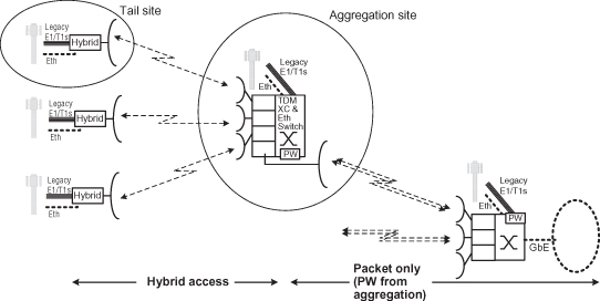
6.5.6 Radio Backhaul Topologies
There are many parameters to be considered when selecting the topology of every network, and even more so when it comes to radio networks, where LOS, rain zone, and other propagation factors should be taken into account—as should aspects such as antenna sites and towers considerations. The common topology choices for radio networks are usually a tree and a ring, or often a combination of both. The tree topology in itself is a combination of two additional basic topologies: the chain and the star, as shown in Figure 6.18.
Figure 6.18. Network topologies.
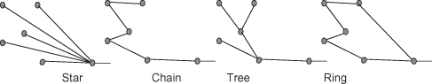
A star topology uses a separate link for each site. This is very simple but not efficient with microwave, because it requires longer radio links and a LOS from origin point to each site, which is unlikely to happen. The star topology also makes for very poor frequency reuse. This is because all the links originate at the same place and the interferences are more likely to happen between links at the same frequency. With chain topology all sites reside on a single path overcoming the star microwave aspects, but resulting in a very sensitive topology where the first link failure causes a complete network failure. Thus almost all links should be protected. Combining the chain and the star yields the tree, at which fewer links can cause major network failures, and only those need to be protected. On the other hand, closing the chain yields the ring, which is the most efficient in terms of protection.
Focusing on the ring and the tree, we will highlight some of these considerations using a simple test case, shown in Figure 6.19. The test case describes a typical radio cluster with one fiber site and 10 cell sites requiring 50 Mbit/s each and aggregated to a total of 400 Mbit/s. Also, it is assumed that every link supporting more than one site needs to be protected. Several aggregation topologies are suggested: tree, single ring, and “tree of rings” (two smaller rings). The tree uses protected links wherever a link failure affects more than a single site.
Figure 6.19. Aggregation topologies test case.
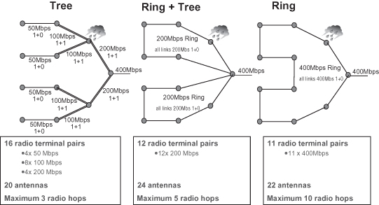
Comparing the network fixed assets cost (CAPEX), we can see that the ring requires fewer radios. On the other hand, more high-capacity radios are needed in a ring, usually at a higher cost and consuming more spectrum. The ring also requires a few more antennas; thus cost comparison is not straightforward and can vary, depending on the particular case. Another factor that can influence cost is spectrum reuse. Since rings have no more than two links at every node, better frequency reuse is usually achieved and often rings are implemented by only a single pair of frequency channels (this depends on the geography of course).
A clear-cut advantage for ring topology is its superior resiliency. The protected tree is indeed protected against equipment failures, but does not provide any path redundancy. Thus it is more vulnerable to heavy fade conditions, as well as to complete site failure (as electricity failure, or weather disaster happens).
Consider the rain situation shown in Figure 6.19; in the case where this site is in complete failure (as a reason of rain, electricity breakdown, or any other failure), it causes the other four sites to fail in the tree, but no other sites in the ring.
The ring also gives a much better availability thanks to its path diversity, because it is necessary for both paths to fail in order to create a service failure. Thus, for achieving the same end-to-end target availability within a tree and a ring, each ring link can be designed for lower availability compared to the tree link. This can save costs through the usage of smaller antennas and lower power at the ring links.
A disadvantage of the ring is that it takes more radio hops to reach the distanced cells. If designed properly, the shortest path can be selected for each traffic flow, but in case of protection where the ring is cut, traffic can flow over N − 1 hops (with N nodes ring). The number of hops can be an issue when considering latency and delay variation, affecting particularly synchronization delivery. Still, when comparing the smaller number of hops in the tree, one should remember that some of them are also with smaller bandwidth than the ring and thus can be with worse performance of delay variation, so this disadvantage is definitely arguable. Limiting the number of maximum hops can be a drive to move into a ring-tree combination, with several smaller rings, as shown in Figure 6.19.
Statistical multiplexing is another advantage of ring topology as derived from the fact that more links share traffic to several sites. On the other hand, since all links are of the same capacity, it may create some disadvantage when adding capacity because all links should be upgraded. This is in contrast to tree topology, where only the tree trunk can be upgraded when adding another branch.
One way to increase ring capacity without upgrading its entire links is to evolve it into a mesh by adding crossing links and breaking it into smaller rings, but this introduces another complexity of managing the connections and protection schemes.
To conclude, there is no single “right” topology. Network planners should consider the particular environmental conditions, business conditions (such as spectrum, radio and antennas costs), reliability requirement, and application characteristics, in order to determine the best solution for their needs.
Backhaul Topology at LTE.
Unlike all prior cellular technologies which are “hub and spoke” networks at which traffic from all RAN-BSs at the cellular sites is aggregated together to the RAN-NC, the LTE defines a flat architecture with direct connectivity between one RAN-BS (called eNB) and its neighbors. Figure 6.20 describes the LTE architecture in comparison to 3G architecture, showing the S1 interface that is toward the core and also showing the X2 interface defined between neighboring eNBs.
Figure 6.20. LTE flat architecture in comparison to 3G architecture.
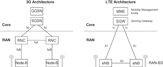
The LTE flat architecture defines actually a mesh mobile backhaul network, but since the X2 interface is used primarily for handoffs (move of a mobile user from one BS to another) with relatively little traffic, it is not likely that the X2 will justify a dedicated physical link. Thus, the mesh connectivity can remain logical but not physical. A logical mesh can be defined over every existing tree or ring topology by creating Ethernet connections such as E-Line or E-LAN.
Note
1 These are physical layer rates. For net traffic rate, one should also consider the Ethernet line overheads.
REFERENCES
1. Infonetics Research, Research Mobile Backhaul Equipment, Installed Base & Services, Copyright 2008, Infonetics Research, Inc.
2. Heavy Reading, Ethernet Backhaul Quarterly Market Tracker, Copyright 2008, Heavy Reading.
3. Heavy Reading, Ethernet Backhaul: Mobile Operator Strategies & Market Opportuni-ties, Copyright 2007, Heavy Reading.
4. Unstrung Insider, Ethernet Microwave: Backhaul & Beyond, Vol. 6, No. 4, April 2007, Copyright 2007, Light Reading.
5. Harvey Lehpamer, Microwave Transmission Networks—Planning, Design and Deployment, McGraw-Hill, New York, 2004.
6. Ethernet ring protection for carrier Ethernet networks, IEEE Commun. Mag., September 2008.
7. ITU-T Rec. G.823, The Control of Jitter and Wander Within Digital Networks which Are Based on the 2048 kbit/s Hierarchy, 2000.
8. ITU-T Rec. G.824, The Control of Jitter and Wander Within Digital Networks which Are Based on the 1544 kbit/s hierarchy, 2000.
9. ITU-T Rec. G.841, Types and Characteristics of SDH Network Protection Architec-tures, 1998.
10. ITU-T Rec. G.8261/Y.1361, Timing and Synchronization Aspects in Packet Networks, 2006.
11. ETSI EN 302 217-2-1 V1.2.1, Fixed Radio Systems; Characteristics and Requirements for Point-to-Point Equipment and Antennas, Part 2-1: System-Dependent Requirements for Digital Systems Operating in Frequency Bands where Frequency Coordination, 2007.
12. ETSI EN 302 217-2-2 V1.2.3, Fixed Radio Systems; Characteristics and Requirements for Point-to-Point Equipment and Antennas, Part 2-2: Harmonized EN Covering Essential Requirements of Article 3.2 of R&TTE Directive for Digital Systems Operating in Frequency Bands where Frequency Co-ordination Is Applied, 2007.
13. ITU-T Rec. G.8032/Y.1344, Ethernet Ring Protection Switching, 2008.
14. ITU-T Rec. G.8031/Y.1342, Ethernet Linear Protection Switching, 2006.
15. ITU-T Draft Rec. Y.1731, OAM Functions and Mechanisms for Ethernet Based Networks, 2006.
16. IEEE Std. 802.1ag, Local and Metropolitan Area Networks, Virtual Bridged Local Area Networks, Amendment 5: Connectivity Fault Management.
17. IEEE Std. 802.1Q, Virtual Bridged Local Area Networks, 2005.
18. MEF 6.1, Ethernet Services Definitions—Phase 2, 2008.
19. MEF 22, Mobile Backhaul Implementation Agreement—Phase 1, 2009.
20. MEF 3, Circuit Emulation Service Definition, Framework and Requirements in Metro Ethernet Networks, 2004.
21. MEF 8, Implementation Agreement for the Emulation of PDH Circuits over Metro Ethernet Networks, 2004.
22. IEEE P802.1ah-2008, IEEE Standard for Local and Metropolitan Area Networks—Virtual Bridged Local Area Networks—Amendment 6: Provider Backbone bridges.
23. IEEE P802.1Qay/D3.0, IEEE Standard for Local and Metropolitan area Networks—Virtual Bridged Local Area Networks—Amendment: Provider Backbone Bridge Traffic Engineering, 18 April 2008.
24. IETF RFC 5086, Structure-Aware Time Division Multiplexed (TDM) Circuit Emulation Service over Packet Switched Network (CESoPSN), 2007.
25. IETF RFC 4553, Structure-Agnostic Time Division Multiplexing (TDM) over Packet (SAToP), 2006.
26. Ceragon Networks, White paper, Flex your backhaul network with adaptive coding & modulation, 2008.