5. Credit Default Swaps
Part I, “What Is Credit Risk?” established the foundations of credit risk, discussing concepts such as default, probabilities of default, and credit spreads. Part II, “Credit Risk Modeling,” then focused on how credit risk models can be used to describe defaults and default probabilities. We focused on the structural approach to credit risk modeling, most notably the Merton model, and also looked at examples of empirical and reduced form models.
In the third and final part of this book, “Typical Credit Derivatives,” we now look at credit derivative instruments that help us manage credit risk. Chapter 2, “About Credit Risk,” contained a quick overview of credit derivatives, and we now focus on two specific instruments: credit default swaps (CDSs) and collateralized debt obligations (CDOs), devoting a chapter to each. As we know from earlier chapters, the main objective of credit derivatives is to transfer credit risk from those that have it but do not want it, to those that are willing to accept it for a fee. In the coming chapters, we are not only going to describe the mechanics of the instruments, but we will also use the credit risk models from Part II to calculate a fair value of that fee.
What Are Swaps?
One of the most fundamental credit derivative instruments in the market is credit default swaps or CDSs. Conceptually, CDSs build on a financial technique known quite simply as a swap. Before we launch into a discussion on CDSs, let’s review the traditional swap.
A swap is exactly what it sounds like: an exchange of one thing for another. In a financial context, the exchange typically consists of one cash flow being exchanged for another cash flow. Put more generally, a financial swap is the exchange of one security’s return for another security’s return. Typical financial swaps include interest rate swaps (where one party normally exchanges a fixed-rate interest stream for another party’s floating-rate interest stream) and total return swaps, where party A pays the total return of a security—for example, the S&P 500—to party B and party B pays the total return of another security—for example, the Nasdaq 100—to party A.
A Typical Swap: Interest Rate Swap
Interest rate swaps are generally used by companies that want to change their exposure to interest rate fluctuations. A company that believes interest rates will drop, and that wants to benefit from that drop, can enter into a swap whereby it exchanges the cash flow of any fixed-rate bonds it has issued for the cash flow of floating-rate bonds. The floating-rate leg of the swap is tied to a reference interest rate in the international financial markets, such as LIBOR.1 The party offering the floating-rate bonds in exchange for the fixed-rate bonds is looking to avoid any exposure to interest rate fluctuations. Generally speaking, a swap can involve any combination of fixed-to-floating, fixed-to-fixed, or floating-to-floating rate.
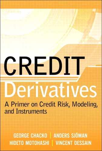
Let’s exemplify. Figure 5-1 shows a swap between AAA Corp and BBB Corp, in which AAA Corp agrees to pay a fixed rate of 5 percent semi-annually on $100 million for three years. In return, BBB Corp agrees to pay the going LIBOR rate semiannually on the same $100 million, also for three years.
Figure 5-1. Diagram of interest rate swap
Every six months for the three years of the swap contract, AAA Corp gives BBB Corp $2.5 million, and BBB Corp gives AAA Corp the amount due given the LIBOR at that time. Practically speaking, the two companies do not exchange the full cash flows. Instead, they determine the difference to see who owes who money. Any actual cash payment between two companies is thus determined by the difference in cash flows. It is this net difference that is actually paid.
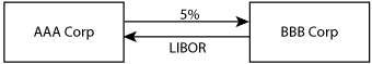
Table 5-1 gives an example of how the cash flow payments could look between the two firms, based on assumptions of how the LIBOR evolved over time. The figure shows the cash flows to BBB Corp from AAA Corp.
Table 5-1. Cash flows for an interest rate swap (from BBB Corp’s perspective)
As the figure shows, after the first six months, AAA Corp owes BBB Corp $2.5 million, and BBB Corp owes AAA Corp $2.3 million, given a LIBOR at the time of 4.6 percent. AAA Corp pays the difference of $0.2 million to BBB Corp. After the next six-month period, LIBOR has increased to 4.7 percent, decreasing the payment from AAA Corp to BBB Corp to $0.15 million. The figure shows the net payments for every period during the three years of the swap contract between the two companies. As it shows, in the end, BBB Corp ends up having paid AAA Corp $0.35 million.
Theoretically, you could swap any type of cash flows. Instead of the interest rates used in the preceding example, you could have a monthly swap of the return of the S&P 500 Index2 for the return on a three-month U.S. Treasury Bill. Each month, you would look at the return of the three-month T-Bill and at the last month’s return on the S&P 500 index, and you would exchange the difference between these two. Put differently, the net receiver is paid by the other party. Because the returns on the S&P 500-index and the three-month T-Bill are expressed in percentage points, the net difference is by default also expressed in percentage points. We want to arrive at a money value, so we multiply the percentage difference by some notional amount. In our previous example of AAA Corp and BBB Corp, the notional amount was $100 million. The size of the notional amount is defined in the swap contract.
A Comment on Pricing Swaps
Our preceding AAA Corp and BBB Corp example covers the mechanics of a swap. However, we left out one important aspect: how to price a swap. Suppose you were asked to pay the return on the S&P 500 in exchange for the one-month return on the three-month T-Bill. (This is the scenario we just described.) Would you be happy with that arrangement as it is or would you like an up-front payment before agreeing to the contract? In other words, what is the fair value of the swap? If it is unfavorable to you to give the counterparty payments based on the S&P 500, the swap has negative value to you and positive value to the counterparty. If it is favorable to you to pay the counterparty based on the S&P 500, the opposite is true.
This example illustrates that every swap has an implicit value to each party. Normally, in a fixed-for-floating swap, the fixed portion—or the fixed leg—is set such that the overall value for both parties is zero. It doesn’t have to be that way, but then one party has to make an up-front payment. If the fixed amount is set too low, the swap has a positive value to the person receiving the floating end, and he has to make an up-front payment to the person receiving the fixed leg to convince him to enter into the swap.
Returning to our S&P 500-for-a-T-Bill example, what is the value of that swap? Should one of the parties make a payment to the other? Most people would guess that the person receiving the S&P 500 returns is better off, because returns on stocks often are higher than the coupons paid on Treasury Bills. However, let’s decompose the swap and fully examine the situation. We know that party A is paying S&P 500 return to party B. In return, party B is paying the one-month return on a three-month U.S.
Treasury Bill. It appears that party A is worse off, and that the swap has negative value to him. If this is true, party A should ask for a compensating up-front payment from party B. However, before we ask party B to pay that fee, let’s look at the swap from another perspective. Imagine that, instead of using a swap, parties A and B do the following: First, party A buys $100 million in S&P 500 stocks and hands that stock over to party B. Party B now receives the return on S&P 500 stocks worth a notional of $100 million. In exchange, party B gives party A $100 million worth of three-month T-Bills. Party A now receives the return on these T-Bills every month, based on a notional of $100 million. We have replicated the swap. We let each party buy $100 million worth of stock or Treasury Bills and hand those securities over to the other party. The replication shows that the swap actually has a value of zero. Each party spends $100 million, which makes them even; it is a fair swap that needs no up-front payment.
Whether or not the stocks will have a higher return than the bonds is of no interest to pricing the swap. However, the difference in return is the speculative basis on which both parties choose to enter the contract; they just happen to take the opposing view on which of the two instruments that will have the higher return. Without different views on that matter, there would be no need for a swap.
Note that our discussion here centers on whether one of the parties wants an up-front payment to enter into the contract. Naturally, a swap generally includes a fee that the protection buyer pays the protection seller; how to determine the fee that is paid for the protection that a CDS gives is the topic of the section “Pricing Single-Name CDSs Using the Structural Approach” later in this chapter.
Credit Default Swaps Defined
Now that we have established how swaps work and introduced their pricing aspect, we are ready to address the focus of this chapter: credit default swaps. Like any swap, the CDS is an exchange of two payments: on the one hand a fee payment and on the other a payment that only occurs if a credit default event happens. As a tool, the CDS is written to cover against the event that an entity or reference asset defaults on its obligations. A comparison with insurance coverage is natural: You pay for home insurance to reimburse any lost value if you are the victim of burglary or damage; and you pay a fee for health and life insurance to pay a sum in the event of injury or death. Insurances use burglary, injury, or death as the events that prompt compensation, where the CDS uses default of the underlying security to trigger payment.3
A Standard Credit Default Swap (CDS)
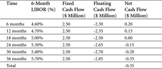
CDSs exist in many variants, and we start with the basic, plain vanilla, credit default swap. The plain vanilla CDS involves two parties that enter into an agreement whereby one party pays the other a periodic fee during a specified time in exchange for a much larger payment should a predefined credit event occur during that time period. If the credit event never occurs, the other party does not have to make any payment. Figure 5-2, repeated from Chapter 2, shows the relationship.
Figure 5-2. Diagram of plain vanilla credit default swap
The fee that the protection buyer pays the protection seller is calculated as a fraction of the notional amount of the reference asset. The fee is often referred to as the credit default swap spread or credit default spread premium, and is paid periodically (monthly, quarterly, semiannually, or yearly).
The credit event is tied to the development of a reference asset such as a bond, loan, or another financial liability. It is easy to think of a typical credit event as a default on a bond, bankruptcy by a firm, or debt restructuring in a company, but the credit event can also be defined more loosely—as a credit spread widening, a rating downgrade, or any other exogenous event. The two swap counterparties can define the credit events as they see fit in the contract that binds them. As an aid, the International Swaps and Derivatives Association (ISDA) has developed standard definitions and documentation to simplify the use of CDSs.
The first party in a CDS swap is looking for protection against a default; we’ll refer to him as the protection buyer or risk hedger. The other party offers that cover for a fee; let’s call her the protection seller or risk buyer. (Returning to the option terminology we developed in Chapter 3, “Modeling Credit Risk: Structural Approach,” the protection buyer could be said to be going short the credit, and the protection seller is going long the credit.)
If the credit event occurs, the CDS contract is terminated and the termination payment takes place. The CDS contract defines one of two payment scenarios. The first option is to use physical settlement, through which the protection buyer has to present the defaulted asset to the protection seller to obtain the termination payment. If a physical settlement is required, the termination payment becomes the full face value of the asset reference. The second option is cash settlement, whereby the protection buyer keeps the asset. In this case, the payment becomes the difference between the face value of the reference asset and its recovery value. The recovery value and the value of the asset after default are then normally assessed by an independent assessor.
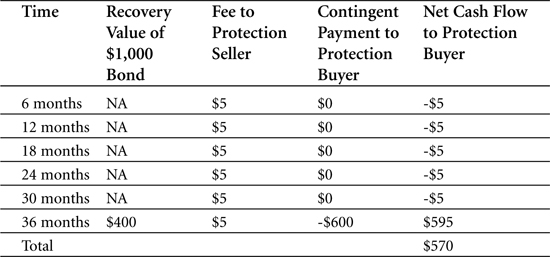
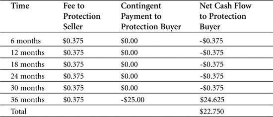
Let’s exemplify. Suppose the protection buyer enters into a five-year CDS for a $1,000 bond. He agrees to pay a semiannual fee of $5 to the protection seller; the fee equals a 1 percent annual premium on the notional amount. In return, the protection seller compensates the protection buyer if the bond issuer fails to make its coupon interest payments. As it turns out, the bond issuer does fail to make coupon payments after three years (or 36 months). Because the CDS contract does not specify physical settlement, an independent party is called to assess the recovery value of the bond. The assessor sets the recovery value to $400. The protection seller then pays the difference between the face value and the recovery value—in this case, $600. (If the contract had specified physical settlement, the protection buyer would have delivered the defaulted asset to the protection seller and received the full face value, $1000, as termination payment.) Table 5-2 outlines the cash flow for this example.
Table 5-2. Cash flows for a plain vanilla CDS ($ million) where default occurs after 36 months
Having looked at the simplest form of a CDS, we can now present some variations on credit default swaps.
Digital Credit Default Swaps
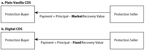
Digital CDSs are almost identical to normal CDSs. The exception is that the recovery rate is fixed beforehand, regardless of the real value of the underlying asset at the time of default. Digital CDSs are therefore also known as fixed-recovery CDSs (and sometimes also referred to as binary CDSs). In other words, the payoff in case of default is independent of the market value of the reference asset at default. Through their construction, digital CDSs eliminate any uncertainty about the recovery rate and the payoff.
Given their distinguishing feature, digital CDSs are typically settled through cash settlement, whereby the protection seller pays out the difference between the asset’s principal value and the predefined recovery value. Studies have shown that the predetermined recovery rate normally ends up being lower than the market value of the asset at the time of default. Expressed differently, the protection buyer receives a larger contingent payment with digital CDSs than for a standard CDS. This increased exposure for the protection seller normally makes the seller ask for a higher fee for a digital CDS than for a standard CDS.
Consequently, the digital credit default swap is normally viewed as more costly in hedging credit risk than a normal CDS.
Figure 5-3 shows the difference of settlement between a plain vanilla CDS and a digital credit default swap.
Figure 5-3. Cash settlement of plain vanilla CDS versus digital CDS
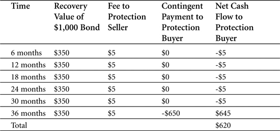
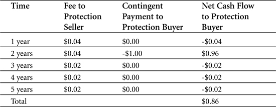
To exemplify how a digital CDS works, we return to our plain vanilla CDS example from earlier. You have just bought protection from a five-year CDS for a $1,000 notional and a 1 percent credit spread. The difference this time is that your digital CDS contract predefines the recovery rate to be $350. After year three, the bond does default on its coupon payments, and the CDS goes into effect. The protection seller pays you the difference between the principal value and the predetermined recovery rate—that is, $650. Table 5-3 outlines the cash flow for this example.
Table 5-3. Cash flows for a digital CDS ($ million) where default occurs after 36 months
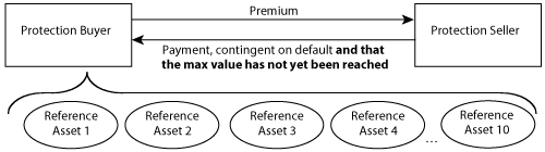
Basket Credit Default Swaps
The plain vanilla CDS we started with in the section “A Standard Credit Default Swap (CDS)” was a single-name CDS, meaning that the CDS contract was written on just one single reference asset. The reference asset can also be a portfolio or group of reference assets such as several bonds or debts. The resulting CDS is then known as a multiname CDS. There exist several types of multiname CDSs; we can think of them as variations on the same CDS theme. One of the more common variations is the basket CDS, where the protection buyer is looking for protection against default on any one of the securities in the basket. A basket swap in which the protection seller has to pay the protection buyer as soon as any of these securities defaults is known as a first-to-default (FTD) basket CDS. The CDS contract may also define a different default security in the basket, such as the second or third security to default. The basket CDS is then known as second-to-default (STD) or third-to-default—and it can more generally be referred to as an nth-to-default basket CDS. As we can see, these variants are similar to the plain vanilla CDS with the exception that the pay-out trigger is the nth credit event in a specified basket of reference entities. Basket CDSs are best suited for protection buyers who may tolerate one or a few defaults, but only up to a certain level.
The basket CDS is a useful instrument for protection buyers looking to shield more than one reference asset from default. As it turns out, the fee on the basket default swap is normally lower than the sum of the fees for individual CDSs on the same reference assets. From a protection seller’s point of view, the basket CDS is also an attractive instrument given the limited exposure to only one of several default probabilities. This leaves the protection seller with the same exposure as in an individual CDS, but on the receiving end of a higher premium fee and thus a higher yield.
Figure 5-4 shows the general structure of a basket CDS and the relationship between the protection buyer and seller.
Figure 5-4. Diagram of a basket default swap
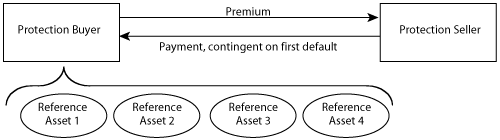
Using the figure, let’s demonstrate how a basket CDS works. Assume that there is a protection buyer who seeks protection against default in any one of four different reference assets. Pooling these together as one group, she looks for a five-year protection scheme. The notional amount for each asset is $25 million and the recovery rates for all assets in this example are (for the sake of simplicity) $0.
The protection buyer enters into a CDS contract with a protection seller, who charges a fee quoted as 3 percent per year, due in semiannual payments. The semiannual payment to the protection seller becomes
![]()
Note that the equation quotes the notional amount of only one asset, rather than that of all four assets. This follows the definition of this particular CDS: It is a first-to-default CDS and thus only covers the first credit event. After a default has occurred, the basket contract is terminated, and the protection buyer stops paying the fee. Like the plain vanilla CDS, settlement can be either physical or cash. In this example, we assume that the contract specifies cash settlement.
Three years into the five-year contract, one of the reference assets defaults. As specified in the contract, the basket CDS expires and the protection seller makes the termination payment. The payment is only for the defaulted asset, because the other reference assets are still non-defaulted and still generate income for the protection buyer. Table 5-4 shows the total cash flows for this basket default swap.
Table 5-4. Cash flows for a basket default swap ($ million)
Portfolio Credit Default Swaps
A portfolio CDS is similar to a basket default swap in that it also references a group of reference assets. However, a portfolio CDS is different from a basket default swap in that it covers a prespecified amount rather than a prespecified sequential default number (first, second, and so on). For example, in a portfolio CDS where the prespecified amount is $10 million and the first default loss is only $5 million, the protection seller pays the $5 million to the protection buyer—and the contract is still active. Just one default does not terminate the contract, unless that default happens to match the predefined amount. A second default with a value of $5 million brings the total default to $10 million, and the contract terminates as soon as the protection seller has paid out the additional $5 million. If the CDS had been a basket swap instead of a portfolio, the contract would have terminated already after the first default.
Figure 5-5 shows a diagram of a portfolio credit default swap. It is almost identical to the diagram of a basket CDS, with the difference that it does not cease to exist until the predefined payment level has been reached.
Figure 5-5. Diagram of a portfolio credit default swap
To exemplify, suppose that the protection buyer in the preceding figure is a bank with a $10 million portfolio, consisting of 10 reference assets, each valued at $1 million with a zero recovery rate. The bank enters a portfolio CDS contract, covering against the first 20 percent default losses in the portfolio. The contract is valid for five years. For this, the bank pays a 2 percent annual premium. In dollars, the premium is calculated as the premium percentage times the covered portion in the portfolio, or
![]()
The protection seller thus receives $40,000 annually in return for covering the first 20 percent of default losses or $2 million.
Now, at the end of year two, one of the reference assets defaults, causing a loss of $1 million. The protection seller pays out the $1 million, but the CDS contract does not expire, because it has not yet reached the $2 million limit. The protection that it provides is still in place, but the premium fee does change, because 10 percent of the default limit has already been paid out. The new premium payment is calculated as
![]()
No more defaults occur after that, and the portfolio CDS expires after five years, as agreed upon in the contract. Table 5-5 shows the total cash flows in this example.
Table 5-5. Cash flows for a basket default swap ($ million)
CDS Indices: iTraxx
Traditionally, traders quote prices, credit spreads, and trading volume of individual CDSs. On an aggregate, indices track the development of prices and volumes for parts or all of the CDS market. Such CDS indices work like all financial indices: Their statistics reflect the combined value of a number of components. Common financial indices are stock market indices, such as the S&P 500 or Dow Jones Industrial Average, which show the composite value of a number of stocks. This value is then often used as a benchmark against which to compare the performance of other instruments or portfolios. More importantly, from a trading point of view, indices can also be used as the underlying collateral against which to write new derivative instruments.
Indices for CDSs were properly introduced in 2003, when investment banks J.P. Morgan and Morgan Stanley launched the market’s first index, known as Trac-X. Trac-X built on the banks’ experience with products known as synthetic TRACERS, tradable baskets of 50 investment-grade CDSs. Soon after the launch of Trac-X, a rival CDS index called iBoxx appeared on the market, launched by a group of American and European banks. In the spring of 2004, Trac-X and iBoxx merged, and management of the new combined index was given to Dow Jones & Company, Inc. The index has since been known as Dow Jones iTraxx (primarily for regional indices for Europe and Asia) or Dow Jones CDS indices (for North America).
The arrival of these CDS indices helped push the market’s liquidity and transparency, because prices and products were now more readily available for all market participants. It also helped widen the product range, because derivative instruments could now be created off the index. Already at the end of their first year of operation in 2003, indices accounted for 11 percent of the credit derivative market in 2003.4
iTraxx contains 125 equally weighted default swaps, composed of both investment grade CDSs and speculative, high-yield CDSs. CDSs are chosen to be part of the index based on their liquidity (the higher their liquidity, the more likely they are to be included in the index), credit quality (a sufficient number of both investment and noninvestment grade CDSs has to be included), and lack of counterparty conflict (CDS issuers that are also large users of the index should not be included in the index, if possible).
Using a Cds Index: A Numerical Example
Just like instruments derived from stock indices, CDS indices are tradable, meaning that they can be used to write derivative instruments. For an iTraxx note, the typical maturity time is between five and ten years, and the notes are normally issued every six months by index note issuer International Index Company Ltd.5 A typical iTraxx note is shown in Figure 5-6.
Figure 5-6. Diagram of iTraxx index note
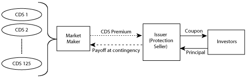
As seen in the figure, investors enter into a contract whereby they receive coupon payments in exchange for paying a principal investment. In case of a default event in one of the underlying CDSs, the issuer pays the investors based on the weight of the defaulted CDS. The contract does not expire, because all the remaining CDSs are still part of the index. However, the principal value of the note does decrease to adjust for the removal of the defaulted CDS. This also affects the coupon payments, which are set as a percentage of the principal.
The left part of Figure 5-6 shows the market maker can view the issuer as a CDS protection seller. The market maker pays the issuer premiums in exchange for a payoff in case one of the reference entities defaults. If a default occurs, the issuer/protection seller then pays the asset’s par value to the market maker while the market maker delivers the actual asset to the issuer. The total notional amount of the index note decreases by the notional amount of the defaulted CDS, and the fee that the protection seller receives is revised accordingly.
For a numerical example, suppose that an issuer launches an iTraxx Europe note with a principal (or par) value of €100 million and a maturity of five years. The note pays a quarterly coupon of three-month Euro LIBOR + 40 basis points (or 0.40 percent) per year on a notional amount of €100 million. We assume that the three-month Euro LIBOR is 4 percent annually, which means that the annual coupon becomes 4.4 percent. In money value, investors who purchase the note then receive a coupon of €4.4 million per year (or €1.1 million every quarter) from the issuer.
The issuer in turn receives a fee from the market maker (the left side of Figure 5-6). We’ll say that this fee is three-month Euro LIBOR plus 36 basis points per year, still on a principal of $100 million. In money terms, the annual fee becomes 4.36 percent times €100 million, or €4.36 million, which per quarter becomes €1.09 million. (The difference of €0.01 million is the loss that the issuer makes on the transaction.)
Now, at the end of year two, a credit event occurs on one of the reference entities in the index. The credit event results in the termination of that CDS, which has been included in the note together with iTraxx’s 125 default swaps, all equally weighted. This gives the defaulted reference entity a weighting of 0.8 percent (or 1/125). We assume that the recovery rate of this particular reference entity is 20 percent. Based on the amount of the asset’s value that can be recovered, the investor is awarded a certain cash settlement. Given the numbers, this settlement becomes:
![]()
The default also means that the notional amount that the investor has put into the note will drop to
![]()
The coupon rate stays the same (three-month Euro LIBOR + 40 basis points per annum) but because the notional amount now has changed, the money value of the quarterly coupon also drops and becomes €1.091 million.
The CDS default also affects the relationship between the issuer (or protection seller) and the market maker that holds the CDSs. The default provokes the contingent payment from the protection seller, calculated as
![]()
In return for the payoff, the market maker delivers the obligations at their face value to the protection seller who can thereby recover as much as possible. From the beginning of year three, the protection sell-er’s notional amount then drops to
![]()
After the default event, the CDS premium remains at 36 basis points on the new notional amount of €99,200,000 until the maturity time of five years. The new quarterly CDS premium payment that the market maker pays the protection seller drops to €1.081 million.
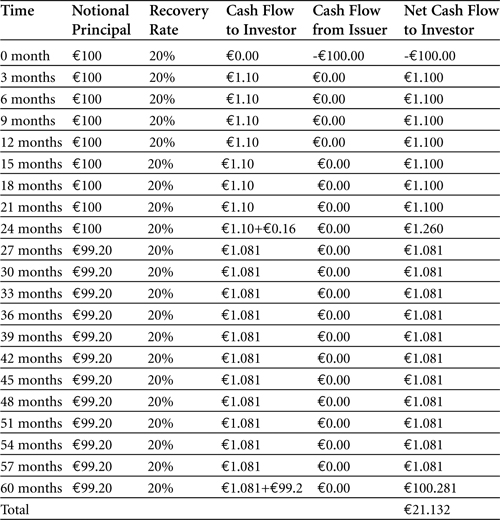
No more credit event occurs after that, and the iTraxx index note expires at maturity after five years. Table 5-6 shows the total cash flows in this example.
Table 5-6. Cash flows for the iTraxx index note (€ million)
Pricing CDSs
From Part II of this book, we know that credit risk models can be divided into structural models, empirical models, and reduced form models. The first two approaches especially help us arrive at probabilities of default for risky debt—and they thus form the basis for pricing the derivative instruments that enable us to transfer credit risk. (As we showed in Chapter 4, “Modeling Credit Risk: Alternative Approaches,” the third approach with empirical models such as the Z-score is best suited for categorizing companies as more or less likely to default. By itself, the approach does not generally produce a default probability for a company or for a liability.)
In this section, we look at how structural and reduced form credit risk models help us price credit default swaps. We first look at how they can be used to price single-name CDSs (swaps written with just one single reference asset as collateral). We then move on to a discussion of various techniques for pricing multiname CDSs (such as basket or portfolio CDSs, which are written on a group of reference assets). Our discussion on multiname CDSs continues in more detail in Chapter 6, “Collateralized Debt Obligations,” which is fully devoted to this particular multiname instrument.
Pricing Single-Name CDSs Using the Structural Approach
When single-name CDSs are priced, the underlying reference asset can be one of many instruments such as a bond, a loan, or any other potentially risky debt. The fee that the protection buyer pays the protection seller is calculated based on the default probability of that one reference asset. As we know by now, we use credit risk models to arrive at default probability values. We’ll now look at how to use both structural and reduced form models to price single-name CDSs, starting with the structural approach.
Pricing CDSs involves making a distinction between the payment stream going from the protection buyer to the protection seller and the stream going in the opposite direction. (Refer to Figure 5-2 for a graphic illustration of the two streams.) Each stream is often referred to as a leg of the CDS. The periodic fee or premium that is paid by the protection buyer is known as the premium leg. The payment that the protection seller has to pay the protection buyer in case of a credit default is called the protection leg. Each leg in the CDS has to be priced individually to come up with the full pricing picture of the CDS.
Pricing the Premium Leg
We start by pricing the premium leg. For this, we need the default probability as defined in the structural approach. Using the Merton model, we recall that default probability, P, in a risk-neutral world can be defined as6
![]()
where the factor d2 is given by
![]()
And where
• N(.) = Cumulative probability distribution function for a standard normal distribution
• D = Debt value
• A0 = Asset value at time 0
• T = Maturity time
• σA = Asset volatility
• r = Risk-free interest rate
We can then convert the probability of default, P, at maturity T years to an annual default probability, called q. Assuming that the annual default probability is constant for each year until maturity, the probability that the obligor will default before maturity can be written as
![]()
Although deriving it is beyond the scope of this book, it can be shown that this probability is in fact the same as the P we defined in equation 8. Hence, we can solve for q and show that it is the same as
![]()
As we now set out to price the premium leg of our single-name CDS, let us look at the cash flow from the protection buyer to the protection seller. We know that this cash flow comes in periodic payments. For simplicity, let’s assume that the payments are annual, denoting them as f, and that they are paid up-front at the beginning of the year. The fee for the first year then becomes f. The fee for the second year becomes the fee times the probability that there has been no default, or f(1-q). For the third year, the fee is f(1-q)2, and so on. Table 5-7 shows the expected fee payment flows.
Table 5-7. Expected fee payment cash flow
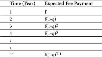
In other words, Table 5-7 shows how we take the expected fee payment for every year between year one and the last year, T. To arrive at the total expected fee payment, we then total up the fee for each year. This can be put into a general formula for the expected total fee payment from a protection buyer to a protection seller as
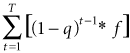
The formula then shows us the cash flows from the premium leg.
Pricing the Protection Leg
Let’s now turn to the cash flows coming from the protection leg, which is the payment that the protection seller has to give the protection buyer if the credit event occurs. Just like the premium leg, the payment leg depends on the probability of default. The final value also depends on how much principal value can be recovered, if a default indeed occurs.
Let’s denote the notional principal of the debt as D. We also denote the recovery rate as q, and we assume that it is constant up until the debt’s maturity. The difference between the two, or 1 – δ, is the loss rate, which we denote as L. The expected loss at default can therefore be expressed as the debt times the loss rate, or
![]()
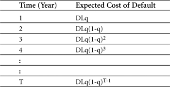
We established in our calculation for the premium leg that the default probability for the first year is q. Adding q to the expected loss at default that we just defined gives us the expected cost for the first year for the protection buyer, or the following:
![]()
Because default in the second year would only occur if default did not happen in the first year, the expected cost in the second year would be
![]()
For all following years up until the year of maturity, T, the expected cost can be computed in the same way. Table 5-8 summarizes the expected costs for various years.
Table 5-8. Expected cost of default
Based on Table 5-8, the expected total cost of default from the protection seller can then be summarized as
![]()
Matching the Premium and Protection Legs
We now have formulas for cash flows for both legs in the credit default swap. For the CDS to be fairly priced, the total fee payment should equal the total default cost. In other words, the formulas for the premium and protection legs should match
Given values of annual default probability, maturity time, risky debt value, and loss rate or recovery rate, the preceding equation can be solved for the expected fee, denoted as f.
A Numerical Example
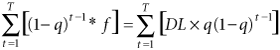
Let’s demonstrate how to price a CDS using the structural approach. Suppose that ABC Corp issues a $100 million bond with a one-year maturity. The bond has semiannual coupon payments, and it is assumed that in case of a default, there is no recovery to be made. To fully paint the scenario, assume further that the current prevailing risk-free interest rate is 5.0 percent. The bond is summarized in Table 5-9.
Table 5-9. ABC Corp’s one-year bond
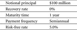
Now, suppose further that there is a bank, Secure Bank Ltd., that buys ABC’s bond and then plans to enter into a CDS contract as protection in case ABC Corp defaults on the bond. (Secure Bank thus becomes the protection buyer.) The CDS premium payments are semiannual, just as for the underlying security. To gather background information on the company, Secure Bank Ltd. studies ABC Corp’s balance sheet, shown in Table 5-10.
Table 5-10. ABC Corp financials (in USD millions)
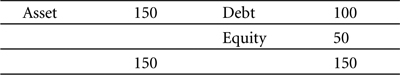
Secure Bank assumes that ABC Corp’s asset volatility is 40 percent.
Secure Bank now needs to determine what a fair price would be for the CDS that it wants to buy. We have all the information we need to calculate the fee that the protection seller is likely to charge, and we start by calculating the default probability for ABC Corp, using earlier equations 8 and 9. They give us
![]()
This default probability is on an annual basis. Because the CDS premium payments are semiannual, the default probability has to be converted into a six-month probability, as follows:
![]()
Based on this default probability, the expected total fee payment, f, to the protection seller—or the premium leg—for two payments (semiannual payments for a one-year maturity) can be calculated using equation 12 as
![]()
We now have the premium leg. Let’s match it with the protection leg payment to obtain a value for f. Given what we know about the CDS from Table 5-9, the expected total contingent payment can be calculated using equation 16. This gives us
![]()
Remember that to arrive at a fair price, the expected total fee payment and expected contingent payment should be equal. Hence, the expected fee payment can be obtained by solving the equation we presented in equation 17.
![]()
$3.7 million is then the total fee that the protection seller will charge for this CDS.
As a final point, we should note a key difference between calculating a credit spread for risky debt and calculating a credit premium for a CDS: The recovery rate is not required for calculating the credit spread according to the Merton model, but is an important input value for calculating the CDS’s credit premium.
Pricing Single-Name CDSs Using the Reduced Form Approach
Let’s now see how we can price a single-name CDS using a reduced form model instead of a structural model. Recall that to produce a credit spread or other price quote, the reduced form model requires default intensity data. (The default intensity value is used to arrive at a default probability, which is the foundation for pricing the derivative.) We’ll apply this knowledge to price the same ABC Corp-based CDS that we just used, and that we defined in Table 5-9. For the reduced form model, we need one additional value that we did not already specify: We will now assume that the default intensity, λ, is constant at 0.05.
Again, we calculate the value of each of the CDS’s two legs, starting with the premium leg. Recall that the probability of default at time t under the simple reduced form approach is given by
![]()
Hence, the probability that ABC Corp will default on its bond at its first payment after six months—or at time t = 0.5—with a default intensity of 0.05, is calculated as
![]()
Because we have assumed that the default intensity is constant over time, the same default probability of 2.47 percent applies for the next six months.
Armed with the default probability for each payment period, we know from equation 20 how to calculate the expected total fee payment to the protection seller. Using our new default probability, we calculate this over two semiannual payments as
![]()
We then calculate the expected total contingent payment just as we did in equation 21. It becomes
![]()
And again, just as before, we match these two formulas, and solve for f.
![]()
The protection fee, using the reduced form approach, is thus $2.5 million.
This value can be compared to the $3.7 million fee that we determined using the structural approach. As we know from earlier chapters, the approaches vary in their approach to determining defaults, and thus a difference in price should be expected. Practically, the structural approach depends much more heavily on balance sheet data than does the reduced form approach. The reduced form approach instead relies on finding a value for default intensity, which as we know from Chapter 4 is rather difficult. If we had assumed a higher or lower value for default intensity in our preceding example, the result would have been quite different—and the difference vis-à-vis the structural model’s result would have changed accordingly. Therefore, we’ll refrain from comparing the two results, because they depend on highly variable inputs to generate their outputs.
Pricing Multiname CDSs: Basic Concepts
We have now looked at how to price credit default swaps that are based on one reference asset. However, as we know from earlier in this chapter, there are several types of CDSs that are based on more than one reference asset. Typical examples of such multiname CDSs are basket and portfolio default swaps. Pricing a multiname CDS is intuitively more complicated than pricing a single-name CDS. First, picture a CDS based on one reference asset. The default pattern for this CDS is easy: It either defaults or it does not. Add one more reference asset, though, and the default pattern immediately gets more complicated: either both reference assets survive, both default, one defaults but not the other, or the other defaults but not the first. In total, there are four possible outcomes. Now, picture a portfolio with ten reference entities. The default pattern has 1,204 possible outcomes (or 210). To price a CDS with this number of possible outcomes using the same technique as for single-name CDSs would require calculating default probabilities for each possible outcome and then adding them up. This would be a rather time-consuming approach. Now, luckily, there exist some statistical techniques that make valuing multiname CDSs easier. We will look at two of these techniques, where the reference assets may or may not be linked to each other. If they are linked, this means that if one asset defaults, several others might be “drawn into” the default as well; we refer to this as default correlation. Calculating the default probabilities of reference assets given their default correlation gives us something known as the loss distribution of the CDS. Both default correlation and loss distribution are important concepts when valuing multiname CDSs, so before we look at how to actually price a multiname CDS, let’s spend some time on these two concepts.
Default Correlation
The distinguishing features of a multiname CDS are that it has more than one reference asset, and that it might face more than one default in any given time horizon. Knowing the probability of any of the underlying entities defaulting lays the groundwork for determining the premium to pay for a multiname CDS. Knowing the probability of more than one default occurring at any given time helps further to set the premium. An even more important measurement is that of how likely two default events are to occur at the same time, known as default correlation. Figure 5-7 gives a visual representation of default correlation.
Figure 5-7. Diagram of default probabilities of two entities
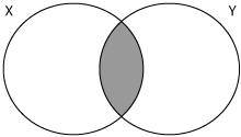
Using the figure, suppose that there are two reference assets, X and Y. The circles X and Y in the preceding figure represent the default probability of assets X and Y, respectively. This default probability can also be denoted as wX and wY. The overlap between the two circles, colored in grey, marks the probability of a joint default, denoted as wX&Y. We can now use these values to create a formula for the probability that X or Y defaults, denoted as wXorY. The formula becomes
![]()
Now, suppose circle X is greater than circle Y, or ωX > ωY. As shown in the left panel of Figure 5-8, if the default correlation is equal to 1, circle X includes the full circle Y. This means that ωX&Y = ωX and ωXorY = ωX. If the default correlation is equal to zero, circle X and circle Y do not share any area, as shown in the right panel of Figure 5-8. This means that ωX&Y is zero and ωXorY = ωX + ωX.
Figure 5-8. Diagram of default probabilities
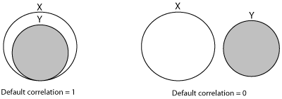
The figure illustrates that the default probability for any of the two individual reference assets increases as default correlation decreases. Applied to a portfolio default swap, for instance, the default probability of the portfolio increases if the default correlation of the two entities approaches zero. There are simply more factors that can cause any one of the assets to default, if the reference assets don’t share the same default factors. This naturally translates into a higher premium to pay for the protection buyer.
Based on equation 28 for ωXorY, it can be shown that the joint default correlation of X and Y, denoted as ρX,Y, can be written as

where the default correlation has to be equal to or larger than -1 and equal to or smaller than 1. (In other words, –1 ≤ρX,Y ≤1.)
Loss Distribution Function
When valuing multiname CDSs, it is also essential to understand the loss distribution function. Let’s use a simple example to explain the loss distribution function by itself (before we add default correlation to the picture). Suppose that we have two reference assets. Asset A has a 100 percent default probability for a loss of 10 percent, and asset B has a 50 percent default probability for two potential losses, one of 5 percent and one of 15 percent. Both assets then have the same average expected loss of 10 percent. However, the losses are distributed differently, which has an effect on the fee that the protection seller wants to charge.
Assume now that our two assets are part of a basket default swap defined as a first-ten-percent loss default swap. For asset A, the protection seller knows she has to compensate for a 10 percent loss with 100 percent probability. For asset B, however, she has a 50 percent probability of a 5 percent loss, and a 50 percent probability of a 15 percent loss. Should the default loss of 15 percent occur, the protection seller does not have to compensate for all 15 percent, because the limit of the contract is set to 10 percent. The default probability of asset B then stays at 50 percent for the same potential loss of 10 percent. Consequently, the protection seller should ask for a lower premium for asset B than for asset A. Despite the fact that the two portfolios have an identical expected loss of 10 percent, the loss distribution gives them different credit spreads.
Let’s look at another example, to which we add the concept of default correlation that we discussed in the previous section. Consider two portfolios that have the same expected loss but different default correlations: one with high default correlation and one with a low default correlation. Figure 5-9 shows possible loss distributions for these two hypothetical portfolios.
Figure 5-9. Loss distribution for two portfolios
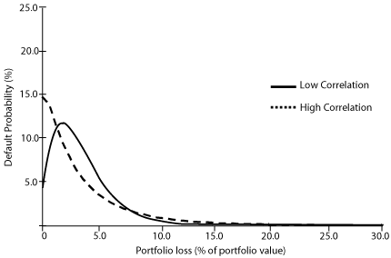
The high correlation portfolio (represented by the dotted line) shows high probability of small losses, with the probability decreasing for higher losses. The low correlation portfolio (shown as the solid line) has a slightly different distribution profile: It has a lower probability than the other portfolio for small losses, but at around the level of 2 percent loss, its probability actually exceeds the high correlation port-folio’s probability. Now, if you were the protection seller, offering a first-two-percent loss basket swap, and the fee payment on both contracts was the same, which portfolio would you choose? Naturally, you’d pick the low correlation portfolio because its probability of loss up to 2.0 percent is smaller than that of the other portfolio.
Pricing Multiname CDSs: A Basket Default Swap
As we just established, both default correlation and loss distribution affect the pricing of a multiname CDS. This section exemplifies how to price a specific type of a multiname CDS, namely the basket default swap. In fact, we use two pricing examples of two completely opposite types of basket default swaps: one with perfect positive correlation between its reference assets and one with zero correlation. In a real-world situation, it would be close to impossible to trade basket CDSs under any one of these two extremes. Most reference assets show some sort of default correlation, and the calculations would have to be adopted to handle such portfolios. Here, however, we satisfy ourselves by looking at these extreme cases, because they help us understand how default correlation affects loss distribution and consequently the CDS protection seller’s payment. We will see how a portfolio with lower correlation has a higher expected loss, and consequently requires a higher fee, than a portfolio with a higher correlation. (These concepts—especially default correlation—are crucial to understanding collateralized debt obligations and are covered more extensively in Chapter 6.)
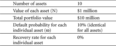
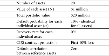
As the basis for both examples, we take a portfolio that consists of ten reference assets. Each reference asset has a value of $1 million, a risk-neutral default probability of 10 percent and a zero recovery rate. The total size of the portfolio ends up as $10 million. Table 5-11 summarizes the portfolio’s profile.
Table 5-11. Portfolio for basket default swaps
Two basket default swaps are written on this portfolio: a first-to-default (FTD) swap and a second-to-default (STD) swap. Their contract term is one year, and we assume for simplicity that default can only occur at the maturity date. We will now calculate the premium fee that the protection sellers of either the FTD or STD swap would charge, for both of the two extreme cases of either full or zero default correlation.
The One Extreme: A Perfect Default Correlation Portfolio
We start with the example of a portfolio with perfect default correlation between its reference assets. Perfect default correlation means that if one reference asset defaults, all reference assets default. This all-forone-and-one-for-all assumption is not far from the behavior of many CDS baskets, where reference entities tend to default or survive together as a group simply because they have similar credit quality.
The general perfect default correlation case can be described as a portfolio composed of N reference assets, where each asset has an individual default probability, ω, that is identical to all other default probabilities in the portfolio over a given time horizon. The notional principal amount of each reference asset, V, is also assumed to be identical. The default event pattern of such a portfolio is simple to describe: Either all reference assets default at the same time, or they don’t. The premium fee that the protection seller requests can then be calculated as expected cost if all assets survive to maturity (survival probability times 0) plus expected cost if all assets default before maturity (default probability times value of each reference asset). Put in a formula, this becomes
![]()
• ω = Individual default probability
• V = Notional principal amount of each reference asset
Using the numbers of our sample portfolio in Table 5-11, the value of each reference asset is $1 million and the default probability is 10 percent. This gives us the information we need to calculate FTD premium fee using equation 30.
![]()
The protection seller is thus likely to charge $100,000 for a CDS written on this particular portfolio.
Theoretically, investors in a second-to-default swap (or any other number-to-default swap) end up paying the same fee as first-to-default swap investors, because the fee is calculated from the individual amount of one reference asset. However, this is based on our assumption of complete correlation; when the first reference asset defaults, the whole portfolio defaults, and thus the risk profile and associated fee is the same no matter which number default the CDS specifies.
The Other Extreme: A Nondefault Correlation Portfolio
The other extreme case for a basket default swap is when there is no default correlation at all between the reference assets. Calculating the premium fee for investors in first- and second-to-default swaps is more complicated than in our perfect default correlation example, because the number of possible default outcomes grows exponentially. In the perfect correlation case, we had two possible outcomes: survival or default of the whole group. In the zero default correlation case, we have the number of reference assets plus one as possible default outcomes. (Either no asset defaults, or one asset defaults, or two default, or....) In our example, this generates 11 possible default outcomes.
Note that one of our assumptions is that defaults can only occur at maturity of the one-year contract. This means that if several defaults happen, they all occur jointly at the same time. We further assume that all assets are identical in terms of asset value and recovery rate. This limits the number of possible default outcomes. If we relaxed this assumption to allow for defaults to occur at any time and for longer maturities, we would theoretically end up with a maximum of 210 or 1,024 possible default outcomes.
The starting point for our price calculation is to find the default distribution of our portfolio; what is the likelihood that we will have between 0 and 10 defaults at the end of the year? If one assumes that the default probabilities follow a binomial distribution, it can be shown that the probability of joint defaults i among N assets in a portfolio, or P(i), can be expressed as
![]()
where
• ω = Individual default probability
• i = Joint default
• i! = i factorial7
• N = Number of assets
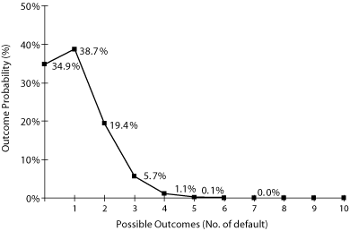
We plug the data that we have about our sample portfolio (as presented in Table 5-11) into equation 32 to calculate the loss distribution of the ten reference assets. For each of the 11 default outcomes (for i=0 to i=10), the equation gives us the probability of that particular outcome. For instance, the probability of one default is 38.7 percent, and that of two simultaneous defaults is 19.4 percent. We then plot all the outcomes on a curve, as in Figure 5-10.
Figure 5-10. Loss distribution with ten reference assets
Using the default distribution, we can complete the picture by looking at the payment that the protection seller has to make in the case of a default. We do this for both our first-to-default and our second-to-default investor. Table 5-12 shows the payments, along with the outcome probabilities represented graphically in Figure 5-10.
Table 5-12. Loss distribution of ten reference assets basket swap
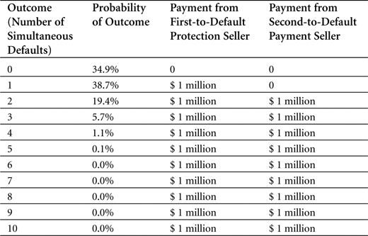
Note how the first-to-default investor or protection seller makes a payment directly when the first default occurs, whereas the second-to-default seller does not pay until at least two defaults occur simultaneously.
We now have the data we need to calculate the actual premium fee that the investors would charge for these basket CDSs. First, let’s establish the formulas needed for both the protection and premium legs of the basket CDS. As the table in Table 5-12 shows us in numbers, the protection payment, given the recovery rate of zero, is equal to the notional amount of one reference asset, V. The expected loss, L, is then calculated as the sum of all outcome probabilities times the reference asset value
![]()
Because the protection leg has to match the premium leg in a CDS, the premium for the first-to-default (FTD) swap should be equal to the expected loss.
![]()
For the second-to-default (STD) swap, the premium should be equal to the expected loss excluding the events of no default and one default.
![]()
Given the loss distribution that we just calculated in Table 5-12, we can calculate the expected loss of the first-to-default swap from equation 33—which is the same as its fee shown in equation 34—and which becomes
![]()
In the same way, the expected loss—and fee—for the second-to-default swap is given by equation 35.
![]()
Comparing the Two Extremes
We have now calculated the prices for two types of basket CDSs (first-and second-to-default) for two default correlation variations on the same basket: either perfect correlation or zero correlation. Table 5-13 summarizes what we have found.
Table 5-13. Summary of expected loss
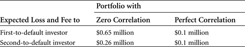
As the preceding table shows, the expected loss—and consequently the fee—of first-to-default swap investors is much lower under perfect correlation than under zero correlation. The same holds true for second-to-default investors. Intuitively, this makes sense: If the entire portfolio behaves as one asset, and all default for the same event, there must be fewer credit factors that can influence the default, and thus less credit risk. The investor or protection seller consequently asks for less of a premium. By contrast, if the reference assets have no default correlation—meaning they all default for different reasons—the level of credit risk increases, because it is more likely that one of the assets—any asset—will default; as a result, the premium fee increases as well.
In the real world, of course, no basket CDSs are based on reference assets with either perfect or zero default correlation. A normal basket CDS has a default probability somewhere between the two extremes, which in turn affects the shape of its loss distribution curve. More advanced statistical approaches than those we have shown here exist for calculating the expected loss and premium fee of these basket CDSs. However, they fall outside of the scope of this book. Our main goal here is to show how the basic concepts of loss distribution and default correlation affect the price of a basket CDS.
Pricing Multiname CDSs: A Portfolio Default Swap
Just as we priced a basket CDS, we will also show how to price another multiname CDS: the portfolio default swap. Recall from earlier in this chapter that the portfolio CDS shares many similarities with the basket CDS, with one major difference: The portfolio CDS covers a prespecified amount rather than a prespecified default number. For example, a first-ten-percent loss portfolio CDS continues to offer protection even after a default occurs, as long as that default has a value that is less than 10 percent of the portfolio. It is when the total default value—irregardless of the number of defaults—reaches 10 percent that the CDS terminates.
We base our example on a portfolio that consists of 20 reference assets, each with a notional amount of $1 million and an individual default probability of 10 percent. We assume that there is zero default correlation between the assets. The portfolio CDS contract is written as a first-10%-loss default swap, and it has a maturity of one year. Table 5-14 summarizes the portfolio’s profile.
Table 5-14. Sample portfolio default swap
Put more generally, our sample portfolio CDS relies on some simplifying assumptions. For instance, the individual default probabilities and notional amounts are treated as identical, and the maturity time is limited to only one time period, with defaults only occurring at the end of that time period. Pricing “real-world” portfolio CDSs, which almost never meet these assumptions, would involve more complicated mathematical operations. Such an example becomes so mathematically complicated that it falls outside of the scope of this book.
Under the preceding assumptions, however, the reference assets in this sample portfolio have the same loss distribution as the basket CDS we priced earlier, because the only difference between them lies in the payoff flows. We can thus reuse equation 32 to calculate the probability of joint default outcomes with i references, denoted as P(i). For simplicity, we repeat that equation:
![]()
where
• ω = Individual default probability
• i = Joint default
• N = Number of assets
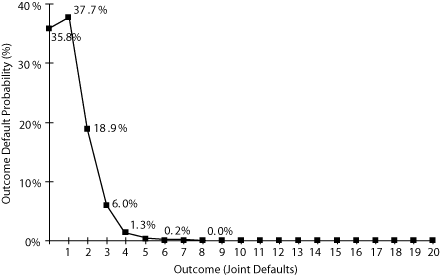
Because the portfolio has 20 reference assets, there are 21 possible default patterns, from no default to 20 joint defaults. Using equation 38, the probability of i simultaneous defaults among 20 assets in a portfolio with individual default probability of 10 percent is calculated as
![]()
For each of our 21 default outcomes (for i=0 to i=20), we use this equation to arrive at a default probability. The result can then be plotted on a loss distribution graph, as shown in Figure 5-11.
Figure 5-11. Loss distribution with 20 reference assets
Now, given the probabilities of joint default outcomes, the expected loss on a portfolio CDS can be calculated by adding up the expected loss for each of the outcomes. For each outcome, the expected loss is calculated as the default probability times the lower of two values: the default value or the remaining value up until the protection cap. As a formula, this gives us
![]()
where
• y = Protection percentage for default loss
• L(i) = Total loss in a portfolio with i defaults
• Min[L(i), NV x y/100] = Selection of the lower value between L(i) and the loss maximum level (expressed as the number of default references, N, times the notional amount, V, times the protection level)
For each of the outcomes, we then calculate the expected loss for the protection seller. Table 5-15 shows the results of those calculations.
Table 5-15. Loss distribution of 20 reference assets portfolio swap
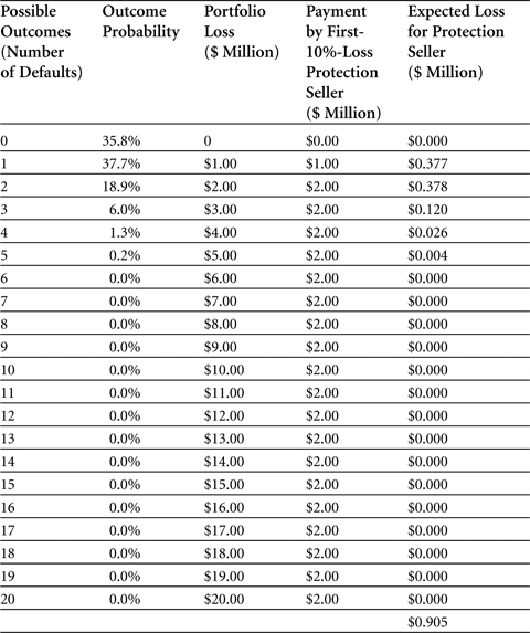
Table 5-15 shows, for each of the outcomes, first the outcome probability (which we saw graphically represented in Figure 5-11) and then the portfolio loss (which is obtained simply by multiplying the number of simultaneous defaults by the notional value of $1 million). The fourth column shows the payment that the protection seller has to make; because the protection is capped at 10 percent of the value of the $20 million portfolio, the payment never exceeds $2 million. The final column shows the expected loss for the protection seller, as computed by multiplying the default probability by the payment. As it turns out, the expected loss value is always lower than the payment. Therefore, we sum up those values to arrive at the total expected loss for the protection seller: $905,000.
As in our basket default swap example, we assume that the expected loss equals the premium fee that the protection seller will charge (for instance, refer to equation 34). In other words, the fee should cover at least the expected loss for the protection seller—who ends up charging a premium fee of $905,000, in this example.
The CDS Market
As we stated in the introduction, a credit default swap can be likened to an insurance policy; it protects against credit events and becomes a sort of default insurance. In theory, any assets that generate cash flows have a credit risk built into them—but they can all be underlined in a CDS. This flexibility, combined with the fact that a CDS can cover any amount and maturity time, explains the growing popularity of the credit default swap as a financial instrument and credit derivative.
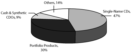
Since 1996, the credit default swap market has seen almost 100 percent annual growth, even during the difficult financial years of the late 1990s. It is by far the largest part of the overall credit derivatives market, as shown in Figure 5-12.
Figure 5-12. Breakdown of credit derivatives market (2003)
Source: Fitch Ratings, as referenced on http://db.riskwaters.com/public/showPage.html?page=168496. Accessed June 2005.
It is worth noting that in addition to having a 47 percent market share in 2003 for single-name default swaps, portfolio products, as well as cash and synthetic8 collateralized debt obligations (CDOs), use default swaps as building blocks for their instruments. In 2003, Fitch Ratings estimated the market for single-name CDSs at $1.9 trillion and portfolio products at $754 billion.9
The trend over the past decade has been to use increasingly diverse asset types as underlying securities for CDSs. According to the British Bankers’ Association (BBA), the major type of underlined assets in 1996 was sovereign debt, which stood at 46 percent. By 2001, the percentage of sovereign debt had decreased to 15 percent as more and more corporate assets were used to create default swaps. Overall, the number of market participants has increased in the past years, resulting in increased liquidity, which in turn has attracted more market participants. The arrival of CDS indices such as iTraxx has also helped to improve the liquidity and transparency of the market.
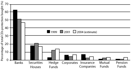
On the buy-side of the market, the largest group of protection buyers using CDSs is the banks. (As you may recall from Chapter 2, banks are the largest protection buyers in the credit derivatives market.) Figure 5-13 shows the overall breakdown of the market by type of protection buyer.
Figure 5-13. CDS protection buyers
Source: Calyon, British Bankers’ Association, Fitch Ratings, as shown on http://db.riskwaters.com/public/showPage.html?page=168229. Accessed June 2005.
Given the importance of CDSs in the credit derivatives market, other leading CDS buyers rank among the major overall buyers in the credit market. What the preceding figure shows is that, except for the top two groups of banks and securities houses, each group’s market share has increased over the past few years. In absolute terms, all groups are buying more, confirming the picture of an increasingly diversified CDS market.
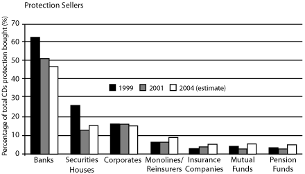
It is clear that banks and other entities operate on both sides of the market. In some cases, they buy protection to transfer default risk off their balance sheets, and in other cases, they act as protection sellers to earn a premium spread. On the sell-side, banks also dominate as sellers of CDS protection. This is shown in Figure 5-14.
Figure 5-14. CDS protection sellers
Source: Calyon, British Bankers’ Association, Fitch Ratings, as shown on http://db.riskwaters.com/public/showPage.html?page=168229. Accessed June 2005.
Endnotes
1 As stated in Chapter 2, LIBOR, London Inter Bank Offered Rate, is the interest rate at which London banks borrow funds from other banks. LIBOR is a widely used reference rate not only for interest rate swaps but also for other derivative instruments such as forward rate agreements.
2 The Standard & Poor’s (S&P) 500 Index is an equity index that measures the collective performance of 500 leading U.S. stock companies. (Other common equity indices include the Dow Jones Industrial Average, the British FTSE 100, or the German Dax 30.) If you invest $1 in the S&P 500 at the start of the month, your monthly return on the S&P 500 would include appreciation in stock prices plus any dividends that are paid during that month, minus the initial $1 dollar.
3 Given this definition, it is worth noting that the credit default swap is not a “pure” swap, because only one of the two cash flows is dependent on an underlying credit security. Several industry participants argue that a CDS could more accurately be referred to as a credit default option (see Janet Tavakoli, “Credit Derivatives and Synthetic Structures” (New York: Wiley, 2001)). However, the nomenclature in the securities market has developed to call even these types of protection-buying instruments for swaps.
4 British Bankers’ Association (BBA), Credit Derivatives Report 2003/2004, page 21.
5 International Index Company Ltd. is a joint venture between several large banks. In June 2005, the financial institutions included ABN Amro, Barclays Capital, BNP Paribas, Deutsche Bank, Deutsche Börse, Dresdner Kleinwort Wasserstein, HSBC, JP Morgan, Morgan Stanley, and UBS Investment Bank.
6 We discussed this in the section, “Using Risk-Neutral Probability to Calculate Default Probability,” in Chapter 3.
7 In mathematics, n! (pronounced n factorial) represents the factorial of a natural number, which is the product of the positive integers less than or equal to n. Here, we use the letter i, but the factorial principle remains the same. For example, if i = 5, then 5! is 5×4×3×2×1 = 120.
8 One way to define CDOs are as cash or synthetic CDOs. If the assets that underlie the CDO are acquired using cash, it becomes a cash CDO. If the assets are acquired by selling protection rather than buying assets, this is seen as a synthetic acquisition, and thus the CDO becomes a synthetic CDO.
9 Fitch Rating’s “Global Credit Derivatives Survey,” September 7, 2004, page 3.