|
In the very act of listening to music, the sound is unconsciously broken down into its component parts by our ear/brain system. But before we can study what the ear does, we must make sure we understand the difference between simple and complex tones.
|
|
|
Sounding the standard A on an electronic oscillator yields what is called a monotone:
|

|
|
The word monotonous, which comes from the words mono and tone, is a good description of this sound—plain and uninteresting.
Sounding the standard A on a good violin yields a much richer sound:
The difference between the pure sine wave of the oscillator and the comparable note of the violin is what music is all about.
The violin has a quality, a timbre, which is pleasing to our ears:
|

|
| The vibration of the violin string itself is a complex process. In fact, it can vibrate at many frequencies at the same time.
|

|
|
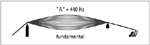
When the tension and length of the string are just right (or in tune, as we would say), bowing the string sets it to vibrating at the standard A, which is defined at 440 vibrations per second, or 440 Hz. This number of vibrations per second is called the fundamental frequency:
|
|
|
Now, the interesting thing is that this same string, with the same tension and length, also vibrates at twice 440 or 880 Hz. The 440-Hz vibration (the fundamental frequency) is called the first harmonic, and the 880-Hz vibration is called the second harmonic:
|

|
|
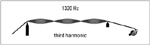
The same bowing action also sets the string to vibrating at three times the fundamental frequency. Three times 440 is 1320 Hz. This is called the third harmonic:
|
|
|
There is also a fourth harmonic at 1760 Hz:
|

|
|
…and a fifth harmonic at 2200 Hz:
…and so on.
|

|
| The fundamental, or first, harmonic, is usually the strongest, and normally the higher the order of the harmonic, the weaker it is.
The harmonic array of the violin tone gives it the richness and specific character which we recognize as coming from the violin. Each instrument in the orchestra has its own particular harmonic signature. The number and relative intensities of these constituent tones determine the quality, or timbre, of that particular instrument.
The wave analyzer is a special electronic instrument that automatically plots the spectrum of any signal applied to its input terminals. For example, the pure 440-Hz tone from the oscillator has no harmonics. All its energy is concentrated at a single frequency:
|


|
|
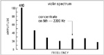
The violin sounding the standard A at 440 Hz, however, has its own characteristic train of harmonics, all of which are multiples of the fundamental:
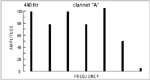
The clarinet sounding an A has the same 440-Hz fundamental followed by its own unique array of harmonics which make it sound like a clarinet: |
|
| The synthesizer can give us an A with almost any harmonic structure desired. Here are two different synthesizer notes, both having 440-Hz fundamentals: |


|
| If we can tell the difference between the sound of the clarinet and the sound of the violin sounding the same note, there is only one conclusion: that the human auditory system can function as a wave analyzer! It is capable of sorting out the harmonics of the violin and clarinet sounds and sensing their relative amplitudes.
|
|
|
Let’s see what each of us can do in “hearing out” the harmonics of the violin A sound. To refresh our memories, here is the violin sound again:
There is no problem recognizing the fundamental, as this is the pitch of the tone:
|

|
|
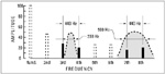
The second harmonic is twice the frequency of the 440-Hz fundamental, or 880 Hz:
|
|
|
Now, as the violin sounds its A, concentrate your attention not on the fundamental but on the 880 Hz, and see if you can hear out that second harmonic. To help calibrate your mind’s frequency scale, an 880-Hz tone will be injected now and then:
|
|
|
It isn’t easy, is it? Don’t be discouraged if you have not made contact yet. This is a rather abstract business, but more chances are coming.
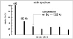
The third harmonic of the violin A falls at 1320 Hz:
|
|
| Let’s see if we can pick out that third harmonic from the violin tone. As before, a tracer tone of 1320 Hz will be injected briefly at times to help us concentrate on that frequency:
|
|
|
Usually, the higher the harmonic, the weaker it is. In spite of this, let’s see what our ears and brains can do on the fifth harmonic of the violin A at 2200 Hz. First, we’ll listen to that frequency to see what it sounds like:
Now, concentrate hard for this fifth harmonic:
|
|
|
With no cue tones for the next 20 seconds, let the personal wave analyzer in your head range up and down the frequency scale to see how many harmonics you can hear out:
We have or at least we have tried to hear out harmonics of the violin tone up to the fifth harmonic. What is the highest harmonic that can be heard? |

|
| Research has shown that a prime requisite of the ability to hear out a harmonic in a complex wave is that the separation between adjacent harmonics must be greater than the critical bandwidth. If two adjacent harmonics fall within a common critical band, the ear cannot distinguish one from the other.
When we consider the seventh and eighth harmonics, we find the critical bandwidth to be about 500 Hz wide. As these harmonics are only separated by 440 Hz, we would expect that the possibility of hearing out the seventh and eighth harmonics would be very small. This is exactly what researchers have found. |
|
| It seems that every time we study a new facet of our hearing, we find critical bands are required to explain it. All this means that the ear is basically like a Fourier analyzer—to use a term familiar to electronics people. We use this analyzing ability of our auditory system all the time without giving it a thought.
In addition to hearing out the harmonics of a complex tone, the ear has remarkable powers of discrimination.
With the people talking all around us, we can direct our attention to one person, subjectively pushing other conversations into the background. We can direct our attention to one group of instruments in an orchestra or to one singer in a choir. Listening to someone talk in the presence of high background noise, we are able to select out the talk and reject, to a degree, the noise. This is all done subconsciously, but we are constantly using this amazing faculty.
We can also use this ability to discriminate between different tones which are close together in frequency. For example, this is our familiar 1000-Hz tone:
|
|
|
This is a tone only 10 Hz higher:
|

|
| We have no difficulty telling the difference between them when we hear them one after the other:
|
|
|
This is 1 percent discrimination.
Can we distinguish tones only 3 Hz apart? Let’s try it:
Most people can tell the difference between the two. This is a discrimination of only three-tenths of 1 percent. All this with common, run of the mill, untrained ears!
|

|
|
How can frequency discrimination of three-tenths of 1 percent be explained? In the first lesson, we were introduced to critical bands. As the widths of critical bands are from 15 to 20 percent of the frequency being considered, at 1000 Hz, the critical band is about 150 Hz wide. How can bands this wide possibly account for frequency discriminations of three-tenths of 1 percent? | |
|
Psychologists have suspected some sort of second filter upstream in the ear/brain system. By inserting microelectrodes into single auditory nerve fibers and then measuring the firing rate of nerve impulses, they found extremely narrow tuning curves. Whether these steep-sided tuning curves are sufficient to explain three-tenths of 1 percent frequency discrimination is still being studied. There may be some time processing as well. At any rate, we stand in awe of the precision the auditory system exhibits.
|

|
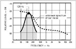
| It is also possible to use the analytical ability of our ears to measure the shape of the spectrum of any common noise, such as this one:
Sound familiar? That noise was recorded in an automobile traveling 55 miles per hour on a freeway. The energy in this noise is distributed throughout the audible spectrum in a way unknown to us. But by using the critical bands in our heads, we shall find out how the energy is distributed from low frequencies to high frequencies.
We’ll make the car our masking noise, and a pure tone will be our exploring probe. First, we will use this 125-Hz tone:
|

|
|
We will adjust the level of the 125-Hz tone until the car noise energy in the critical band centered on this frequency just masks the tone:
The level of the tone is now -15 dB. The tone is clearly audible in the car noise, so we’ll reduce the level of the tone by 5 dB:
The tone can still be heard, but we are closer to the point at which the car noise masks the tone. I shall now reduce the level of the tone until it is just masked by the noise as I hear it:
Now, the level of the tone is about -23 dB. To my ears, this is the masking threshold at 125 Hz. You may or may not agree with me, but we are illustrating a principle rather than trying for precise, universal results. Each set of ears is unique, and differences are to be expected.
|
|
| But let’s go on to another frequency, 500 Hz:
The 500-Hz tone is clearly audible in the car noise. Now, we’ll decrease the level of the tone 5 dB:
The tone is still audible, so let’s reduce it until it is just masked by the car noise in the critical band centered on 500 Hz:
|

|
|
There. To my ears, the tone reaches threshold at a level of -44 dB. That is a second point on our curve.
For a third point on our car noise spectrum curve, let us use a probe tone of 2000 Hz:
|

|
|
Now, the 2000-Hz probe tone level will be gradually reduced until it is just masked by the car noise:
For me, the level of the 2000-Hz tone is -46 dB at threshold. We now have three points on our car noise spectrum curve. We find that as frequency is increased, the energy level of the car noise tends to fall off. This is typical of many noises in our environment. Now many other points could be plotted to reveal greater detail of the shape of our car noise spectrum.
|

|
| We must call this a critical band spectrum because each point is dependent upon the width of the critical band at each measuring frequency. Its shape will be very close to that of a spectrum measured with a one-third octave analyzer because critical bandwidths are not too far from one-third octave bandwidths.
We must pause here to reconsider the significance of what we have just done. We have determined the spectral shape of a common environmental noise by using the critical bands in our auditory system as the analyzer. This is based on the principle that only the noise energy within the critical band centered on the probe tone frequency is effective in masking the tone.
So, what have we done? We have demonstrated the remarkable analytical ability of our hearing system—an ability which we use all the time without giving it a second thought. And that isn’t all. Other equally astounding characteristics of the human ear will be demonstrated in future lessons.
|
|