
Chapter 11
Split-Plot Designs to Accommodate Hard-to-Change Factors
Oftentimes, complete randomization of all test parameters is extremely inefficient, or even totally impractical.
Alex Sewell
53rd Test Management Group, 28th Test and Evaluation Squadron, Eglin Air Force Base
Researchers often set up experiments with the best intentions of running them in random order, but they find that a given factor, such as temperature, cannot be easily changed, or, if so, only at too much expense in terms of time or materials. In this case, the best test plan might very well be the split-plot design. A split plot accommodates both hard-to-change (HTC) factors, e.g., the cavities in a molding process, and those that are easy to change (ETC); in this case, the pressure applied to the part being formed.
How Split Plots Naturally Emerged for Agricultural Field Tests
Split-plot designs originated in the field of agriculture where experimenters applied one treatment to a large area of land, called a whole plot, and other treatments to smaller areas of land within the whole plot, called subplots. For example, when D. R. Cox wrote about the “Split Unit Principle” in his classic Planning of Experiments (John Wiley & Sons, 1958), he detailed an experiment on six varieties of sugar beets (number 1 through 6) that are sown either early (E) or late (L). Figure 11.1 shows the alternatives of a completely randomized design versus one that is split into two subplots.
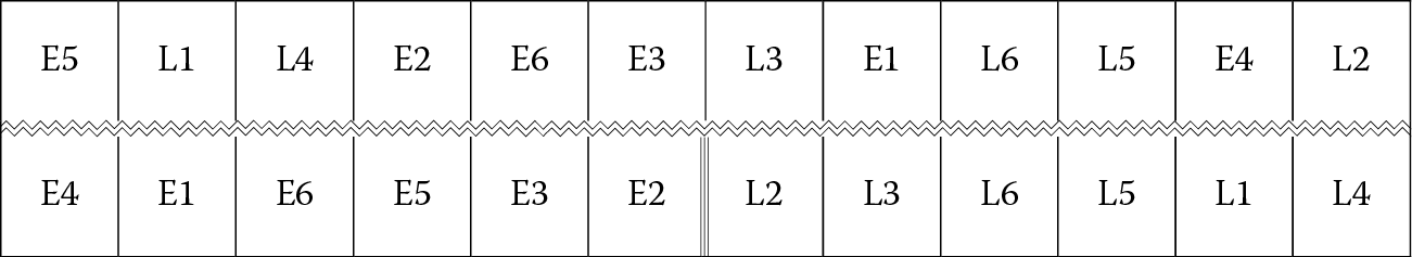
A completely randomized experiment (top row) versus one that is divided into split plots (bottom row).
The split-plot layout made it far easier to sow the seeds because of the continuity in grouping. This is sweet for the sugar beet farmer (pun intended). However, as with anything that seems too easy, there is a catch to the more convenient test plan at the bottom of Figure 11.1: It confounds the time of sowing with the blocks of land, leaving no statistical power for assessing this factor (early versus late). The only way around this is to replicate the whole plot, that is, repeat this entire experiment on a number of fields, as is provided in another agricultural split plot illustrated by Figure 11.2. It lays out a classic field study on three varieties (V) of oats treated with four levels of nitrogen (N) fertilizer described by Sir Fisher’s protégé (DOE pioneer Frank Yates. 1935. Complex experiments. Journal of the Royal Statistical Society Supplement 2: 181–247). The varieties were conveniently grouped into randomized whole plots within six blocks of land (we only show three blocks). It was then fairly easy to apply the different fertilizers chosen at random.

Applying a Split Plot to Save Time Making Paper Helicopters
Building paper helicopters as an in-class design of experiments (DOE) project is well established for a hands-on learning experience (see, for example, George’s Column: Teaching Engineers Experimental Design with a Paper Helicopter, by George Box. 1992. Quality Engineering 4 (3): 453–459). Figure 11.3 pictures an example—the top flyer from the trials detailed in this case study.

Inspired by news of a supreme paper (Conqueror CX22) made into an airplane that broke the Guinness World Record™ for greatest distance flown (detailed by Sean Hutchinson in The Perfect Paper Airplane, Mental Floss, January 14, 2014), engineers at Stat-Ease (Mark and colleagues) designed a split-plot experiment on paper helicopters. They put CX22 to the test against a standard copy paper. As laid out below, five other factors were added to round out the flight testing via a half-fraction, high-resolution (Res VI) two-level design with 32 runs (= 26-1):
- Paper: 24# Navigator Premium (standard) versus 26.6# Conqueror CX22 (supreme)
- Wing (technically a rotor in aviation terms) Length: Short versus Long
- Body Length: Short versus Long
- Body Width: Narrow versus Wide
- Clip: Off versus On
- Drop: Bottom versus Top
Being attributes of construction, the first four factors (identified with lower-case letters) are hard to change, i.e., HTC. The other factors come into play in the flights (operation). They are easy to change (ETC).
To develop the longest flying, most-accurate helicopter, the experimenters measured these two responses (Y):
- Average time in seconds for three drops from ceiling height
- Average deviation in centimeters from target
The averaging dampened out drop-to-drop variation, which, due to human factors in the release, air drafts, and so forth, can be considerable.
The experimenters enlisted a worker at Stat-Ease with the patience and skills needed for constructing the paper helicopters. Grouping the HTCs number of flying machines into whole plots, as shown in Table 11.1, reduced the manufacturing time by one half.
Partial listing (first three groups and the last) of 32-run split-plot test plan
|
Group |
Run |
a: Paper |
b: Wing |
c: Body Length |
d: Body Width |
E: Clip |
F: Drop |
|
1 |
1 |
Nav Ultra |
Long |
Short |
Narrow |
Off |
Top |
|
1 |
2 |
Nav Ultra |
Long |
Short |
Narrow |
On |
Bottom |
|
2 |
3 |
CX22 |
Short |
Short |
Narrow |
Off |
Top |
|
2 |
4 |
CX22 |
Short |
Short |
Narrow |
On |
Bottom |
|
3 |
5 |
Nav Ultra |
Long |
Long |
Narrow |
Off |
Bottom |
|
3 |
6 |
Nav Ultra |
Long |
Long |
Narrow |
On |
Top |
|
… |
… |
… |
… |
… |
… |
… |
… |
|
16 |
31 |
CX22 |
Short |
Long |
Wide |
Off |
Top |
|
16 |
32 |
CX22 |
Short |
Long |
Wide |
On |
Bottom |
After the 16 helicopters were built (numbered by group with a marker), the engineers put each one (in run order) to the test with combinations of the two ETC factors as noted in the table.
Trade-Off of Power for Convenience When Restricting Randomization
As shown in Table 11.2, of the two responses, the distance from target (Y2) produced the lowest signal-to-noise ratio. It was based on a 5-cm minimal deviation of importance relative to a 2-cm standard deviation measured from prior repeatability studies.
Signal-to-noise for the two paper helicopter responses
|
Response |
Signal |
Noise |
Signal/Noise |
|
Time avg |
0.5 sec |
0.15 sec |
3.33 |
|
Target avg |
5.0 cm |
2.00 cm |
2.50 |
Assuming a whole-plot to split-plot variance ratio of 2 (see boxed text below: Heads-Up about Statistical Analysis of Data from Split Plots, for background), a 32-run, two-level factorial design generates the power shown in Table 11.3 at 2.5 signal-to-noise for targeting.
Power for main effects for design being done as split plot versus fully randomized
|
Design |
Hard (a–d) |
Easy (E, F) |
|
Split plot |
82.1% |
99.9% |
|
Randomized |
97.5% |
97.5% |
What’s really important to see here is that, by grouping the HTC factors, the experimenters lost power versus a completely randomized design. (It mattered little in this case, but it must be noted that the other factors (the ETCs) gained a bit more power, going from 97.5% to 99.8%.) However, the convenience and cost savings (the CX22 stock being extremely expensive) of only building half the paper helicopters—16 out of the 32 required in the fully randomized design of experiments—outweighed the loss in power, which in any case remained above the generally acceptable level of 80%. Thus, the split-plot test plan laid out in Table 11.1 got the thumbs up from the flight engineers.
Much more could be said about split plots and the results of this experiment in particular (for what it’s worth, CX22 did indeed rule supreme). The main point here is how power was assessed to “right size” the test plan while accommodating the need to reduce the builds.
One More Split Plot Example: A Heavy-Duty Industrial One
George Box in a Quality Quandaries column on Split Plot Experiments (Quality Engineering, 8(3), 515–520, 1996) detailed a clever experiment that discovered a highly corrosion-resistant coating for steel bars. Four different coatings were tested (easy to do) at three different furnace temperatures (hard to change), each of which was run twice to provide power. See Box’s design (a split plot) in Table 11.4 (results for corrosion resistance shown in parentheses). Note the bars being placed at random by position.
Split plot to increase corrosion resistance of steel bars
|
Group |
Heats (Deg C) (Whole plots) |
Positions (Subplots) |
|||
|
1 |
360 |
C2 (73) |
C3 (83) |
C1 (67) |
C4 (89) |
|
2 |
370 |
C1 (65) |
C3 (87) |
C4 (86) |
C2 (91) |
|
3 |
380 |
C3 (147) |
C1 (155) |
C2 (127) |
C4 (212) |
|
4 |
380 |
C4 (153) |
C3 (90) |
C2 (100) |
C1 (108) |
|
5 |
370 |
C4 (150) |
C1 (140) |
C3 (121) |
C2 (142) |
|
6 |
360 |
C1 (33) |
C4 (54) |
C2 (8) |
C3 (46) |
The HTC factor (temperature) creates so much noise in this process that in a randomized design it would overwhelm the effect of coating. The application of a split plot overcomes this variability by grouping the heats, in essence, filtering out the temperature differences. The effects graph in Figure 11.4 tells the story.
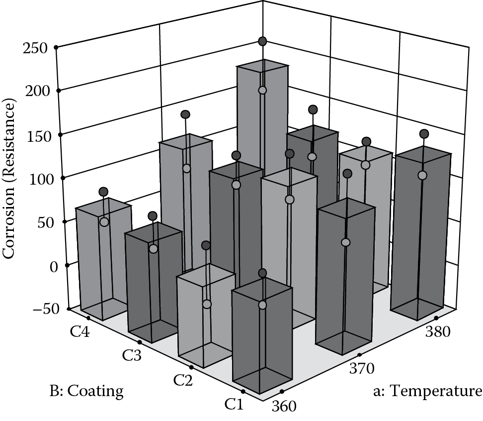
The combination of high temperature with coating C4, located at the back corner, towers above all others. This finding, the result of the two-factor interaction aB between temperature and coating, achieved significance at the p < 0.05 threshold. The main effect of coating (B) also came out significant. If this experiment had been run completely randomized, p-values for the coating effect and the coating-temperature interaction would have come out to approximately 0.4 and 0.85 p-values, respectively, i.e., nowhere near to being statistically significant. Box concludes by suggesting the metallurgists try even higher heats with the C4 coating while simultaneously working at better controlling furnace temperature. Furthermore, he urges the experimenters to work at understanding better the physiochemical mechanisms causing corrosion of the steel. This really was the genius of George Box—his matchmaking of empirical modeling tools with subject matter expertise.
Our brief discussion of split plots ends on this high note.
Must We Randomize Our Experiment?*
DOE guru George Box addressed this frequently asked question in his 1989 report: “Must We Randomize Our Experiment” (#47, Center for Quality and Productivity Improvement, University of Wisconsin/Madison), advising that experimenters:
- Always randomize in those cases where it creates little inconvenience.
- When an experiment becomes impossible, being subjected to randomization, and you can safely assume your process is stable, that is, any chance variations will be small compared to factor effects, then run it as you can in nonrandom order. However, if due to process variation, the results would be “useless and misleading” without randomization, abandon it and first work on stabilizing the process.
- Consider a split-plot design.
“Designing an experiment is like gambling with the devil: only a random strategy can defeat all his betting systems.”
Sir Ronald A. Fisher
* Excerpted from StatsMadeEasy blog 12/31/13 www.statsmadeeasy.net/2013/12/must-we-randomize-our-experiment/
Report from the Field
Paul Nelson (Ph.D., C.Stat.) in a private correspondence to the authors passed along this story of his exposure to split-plot experimentation from where these first sprung up:
The Classical (agricultural) Experiments conducted at Rothamsted Agricultural Research Station, Harpenden, United Kingdom (www.rothamsted.ac.uk), are the longest running agricultural experiments. Of the nine started between 1843 and 1856, only one has been abandoned. Unfortunately, we had to wait until the 1920s before the introduction of factorial treatment structures, so the designs are simple and follow the one-factor-at-a-time (OFAT) dictum. What is fascinating about these experiments is the clearly visible lines between strips, plots, and subplots of land due to the treatments (species, fertilizers, nitrogen sources, etc.) applied. The Rothamsted Classical Experiments are described in detail and beautifully illustrated in a document online at www.rothamsted.ac.uk/sites/default/files/LongTermExperiments.pdf.
The first split-plot experiment I came across was as an undergraduate student. My soon-to-be PhD supervisor, Rosemary Bailey (later professor of Statistics and head of the School of Mathematical Sciences at Queen Mary, University of London), who at the time was still working at Rothamsted, was the lecturer. The experiment was the comparison of three different varieties of rye grass in combination with four quantities of nitrogen fertilizer. The two fields of land (replicate blocks) were each divided into three strips (whole plots) and each strip divided into four subplots per strip. The rye grass varieties were sown on the strips by tractor, whilst the fertilizers could be sown by hand on the subplots. The response was percent dry-matter harvested from each plot.
Straying from Random Order for the Sake of Runnability
Observe in this experiment design layout (Table 11.4) how Box made it even easier, in addition to grouping by heats, by increasing the furnace temperature run-by-run and then decreasing it gradually. This had to be done out of necessity due to the difficulties of heating and cooling a large mass of metal. The saving grace is that, although shortcuts like this undermine the resulting statistics when they do not account for the restrictions in randomization, the effect estimates remain true. Thus, the final results can still be assessed on the basis of subject matter knowledge as to whether they indicate important findings. Nevertheless, if at all possible, it will always be better to randomize levels in the whole plots and, furthermore, reset them when they have the same value, e.g., between Groups 3 and 4 in this design.
“All industrial experiments are split plot experiments.”
Cuthbert Daniel
Heads-Up about Statistical Analysis of Data from Split Plots
Split plots essentially combine two experiment designs into one. They produce both split-plot and whole-plot random errors. For example, as pointed out by Jones and Nachtsheim in their October 2009 primer on Split-Plot Designs: What, Why, and How (Journal of Quality Technology 41 (4)), the corrosion-resistance design introduces whole-plot error with each furnace reset due to variation by operators dialing in the temperature, inaccurate calibration, changes in ambient conditions, and so forth. Split-plot errors arise from bad measurements, variation in the distribution of heat within the furnace, differences in the thickness of the steel-bar coatings, and so forth.
This split error-structure creates complications in computing proper p-values for the effects, particularly when departing from a full-factorial balanced and replicated experiment, such as the corrosion-resistance case. If you really must go this route, be prepared for your DOE software applying specialized statistical tools that differ from standard analysis of variance (ANOVA). When that time comes, take full advantage of the help provided with the program and do some Internet searching on the terms. However, try not to get distracted by all the jargon-laden mumbo jumbo that may appear in the computer output; just search out the estimated p-values and thank goodness for statisticians and programmers who sort this all out.
“If the Lord Almighty had consulted me before embarking on Creation, I should have recommended something simpler.”
Alphonso the Wise (1221–1289)