The Difference Between Statsmodels and Prophet

Time-series analysis typically requires missing values and outliers diagnosis and treatment, multiple test statistics to verify key assumptions, hyperparameter optimization, and seasonal effects control. If we commit a slight mistake in the workflow, then the model will make significant mistakes when forecasting future instances. Consequently, building a model using Statsmodels reasonably requires a certain level of mastery.

Fondly remember that machine learning is about inducing a computer with intelligence using minimal code. Statsmodels does not offer us that. Prophet fills that gap. It was developed by Facebook’s Core Data Science team. It performs tasks such as missing value and outlier detection, hyperparameter optimization, and control of seasonality and holiday effects. To install FB Prophet in the Python environment, use pip install fbprophet. To install it in the Conda environment, use conda install -c conda-forge fbprophet.

Understand Prophet Components

In the previous chapter, we painstakingly built a time-series model with three components, namely, trend, seasonality, and irregular components.

Prophet Components

The Prophet package sufficiently takes into account the trend, seasonality and holidays, and events. In this section, we will briefly discuss the key components of the package.

Trend

A trend is a single and consistent directional movement (upward or downward). We fit a time-series model to discover a trend. Table 4-1 highlights tunable trend parameters.

Table 4-1

Tunable Trend Parameters

Parameters	Description
growth	Specifies a piecewise linear or logistic trend
n_changepoints	The number of changes to be automatically included, if changepoints are not specified
change_prior_scale	The change of automatic changepoint selection

Changepoints

A changepoint is a penalty term. It alters the behavior of a time-series model. If you do not specify changepoints, the default changepoint value is automated.

Seasonality

Seasonality represents consistent year-to-year upward or downward movements. Equation 4-1 approximates this.

(Equation 4-1)

Here, P is the period (7 for weekly data, 30 for monthly data, 90 for quarterly data, and 365 for yearly data).

Holidays and Events Parameters

Holidays and events affect the time series’ conditional mean. Table 4-2 outlines key tunable holiday and event parameters.

Table 4-2

Holiday and Event Parameters

Parameters	Description
daily_seasonality	Fit daily seasonality
weekly_seasonality	Fit weekly seasonality
year_seasonality	Fit yearly seasonality
holidays	Include holiday name and date
yeasonality_prior_scale	Determine strength of needed for seasonal or holiday components

The Additive Model

The additive models assume that the trend and cycle are treated as one term. Its components are similar to the Holt-Winters technique. We express the equation as shown in Equation 4-2.

(Equation 4-2)

The formula is written mathematically as shown in Equation 4-3.

(Equation 4-3)

Here, g(t) represents the linear or logistic growth curve for modeling changes that are not periodic, s(t) represents the periodic changes (daily, weekly, yearly seasonality), h(t) represents the effects of holidays, and + ?_? represents the error term that considers unusual changes.

Develop the Prophet Model

Forecast

Listing 4-5 applies the predict() method to forecast future instances.

forecast = m.predict(future)

Listing 4-5

Forecast Time Series

Listing 4-6 plots previous values and forecasted values (see Figure 4-1).

m.plot(forecast)

plt.xlabel("Date")

plt.ylabel("Price")

plt.xticks(rotation=45)

plt.show()

Listing 4-6

Forecast

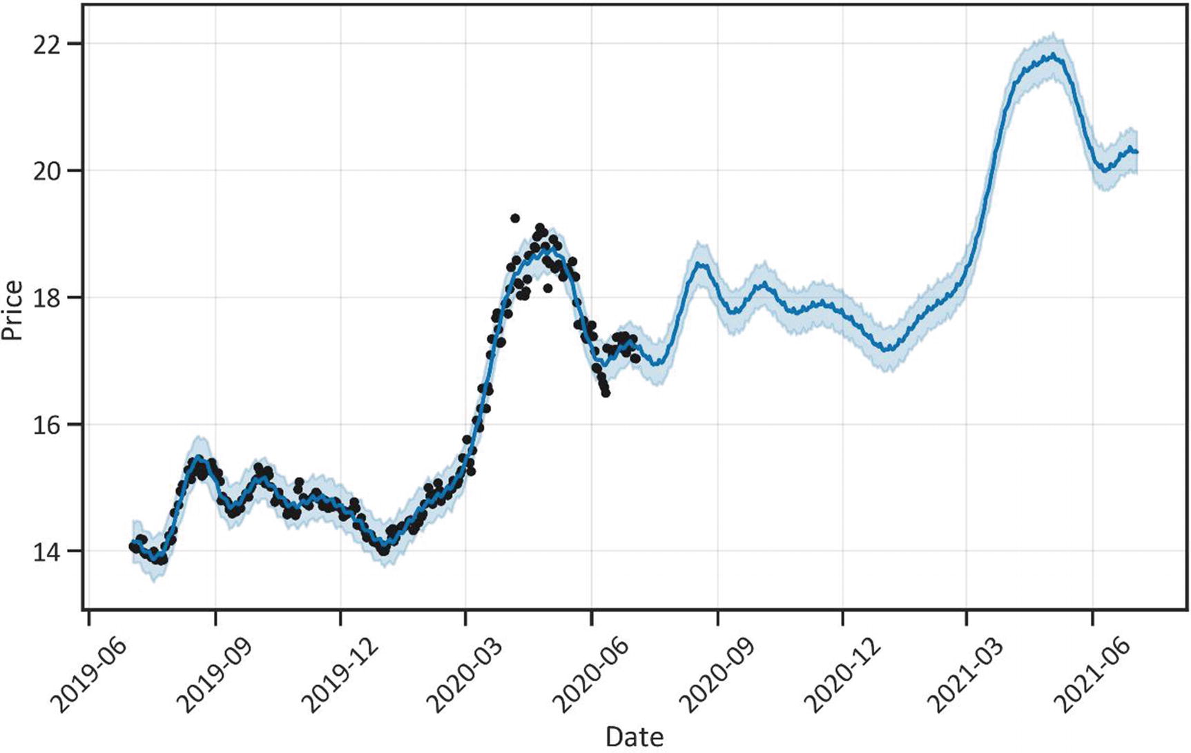
Figure 4-1 tacitly agrees with the SARIMAX in the previous chapter; however, it provides more details. It forecasts a long-run bullish trend in the first quarters of the year 2021.

Seasonal Components

Listing 4-7 decomposes the series (see Figure 4-2).

model.plot_components(forecast)

plt.show()

Listing 4-7

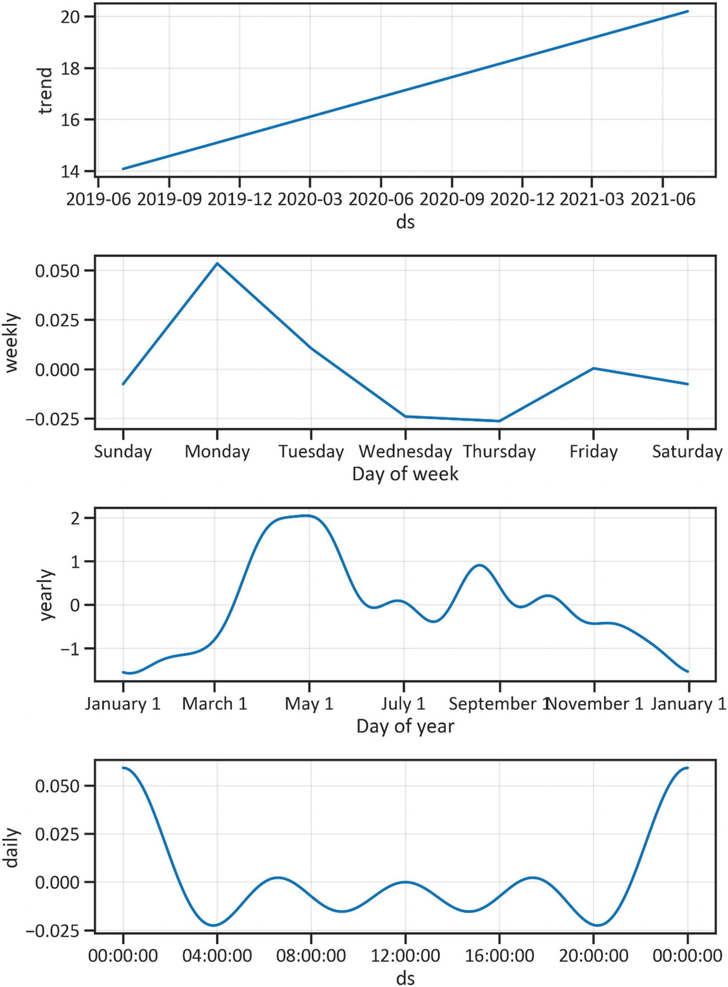
Seasonal Components

Cross-Validate the Model

Evaluate the Model

Conclusion

This chapter covers the generalized additive model. The model takes seasonality into account and uses time as a regressor. Its performance surpasses that of the seasonal ARIMA model. The model commits minor errors when forecasting future instances of the series. We can rely on the Prophet model to forecast a time series.

The first four chapters of this book properly introduce the parametric method. This method makes bold assumptions about the underlying structure of the data. It assumes the underlying structure of the data is linear.

The subsequent chapter introduces the nonparametric method. This method supports flexible assumptions about the underlying structure of the data. It assumes the underlying structure of the data is nonlinear.