In the previous chapter, we discussed Azure Machine Learning service tools, functionality, and assets. This chapter focuses on providing hands-on experience to users and develop end-to-end machine learning project life cycle using Azure ML SDK. As mentioned in the previous chapter, Azure ML offers Python SDK, R SDK, and low-code or zero-code Azure ML designer approaches to develop, train, and deploy ML models; we will use Python SDK for our hands-on labs in this chapter. For the purposes of hands-on lab in this chapter, we will assume users are familiar with Python and getting started with implementing data science solutions on cloud.
Lab setup
Let’s get started with setting up the lab environment! To follow the hands-on lab in this chapter, users need to have an Azure subscription. Users can also sign up for a free Azure subscription worth $200 here (https://azure.microsoft.com/en-us/free/). After signing up, users will be able to create Azure ML service from the portal (https://portal.azure.com/) or Azure gov portal (https://portal.azure.us).
Azure ML is currently available in two Azure Government regions: US Gov Arizona and US Gov Virginia with basic edition being generally available and enterprise edition in preview. The service in Azure Government is in feature parity with Azure commercial cloud. Refer to this link for more info: https://azure.microsoft.com/en-us/updates/azure-machine-learning-available-in-us-gov/.
Bank marketing dataset posted here (https://github.com/singh-soh/AzureDataScience/tree/master/datasets/Bank%20Marketing%20Dataset). Original source www.kaggle.com/janiobachmann/bank-marketing-dataset.
Compute instance as development environment (note: as explained in the previous chapter, users can also use local computer, DSVM, or Databricks). Azure ML SDK needs to be installed when working on local or in Databricks; please follow the instructions here to set up in your local environment/Databricks:
https://docs.microsoft.com/en-us/azure/machine-learning/how-to-configure-environment
JupyterLab notebooks (already installed on compute instance).
Azure ML extension is also available if you prefer visual studio code. The extension supports Python features as well as Azure ML functionalities to make the development environment handier. Refer here to install the extension:
https://marketplace.visualstudio.com/items?itemName=ms-toolsai.vscode-ai
- 1.
From the Azure portal, type “Machine Learning” (without quotes) in the search box at the top of the page.
- 2.
Click Machine Learning in the search results.
- 3.
Click + Add.
- 4.
Create a new resource group or select an existing one.
- 5.
Provide a name for the Azure ML workspace.
- 6.
For location, select a region closest to you.
- 7.
For workspace edition, select Enterprise edition. We will use Enterprise edition for the hands-on lab. Building AutoML experiments on Azure ML Studio is not supported in basic edition. Please refer to here to see capabilities in basic and enterprise edition:
https://docs.microsoft.com/en-us/azure/machine-learning/concept-editions
- 8.
Click Review + Create, and then click Create in the subsequent screen.
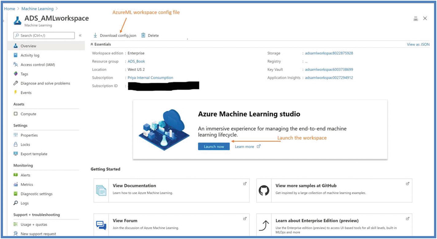
Azure ML workspace on Azure PortalClick on “Launch now” to launch the workspace. Once the workspace is launched, you will see the workspace as shown in Figure 5-2

Azure ML Studio workspace
In the previous chapter, we covered all the assets and concepts of Azure ML workspace. In this chapter, we will use those assets to build our analysis on bank marketing dataset.
Getting started with JupyterLab
- 1.
Click Compute.
- 2.
Under Compute Instance, create a new compute instance without any advanced settings (explained in Chapter 4, Figure 4-9).
- 3.
Once compute instance is created, click JupyterLab to launch it.
- 4.
Under Users, click your name and create a folder called “BankMarketingAnalysis.”
- 5.Under “BankMarketingAnalysis Folder,” create a Python 3.6 Azure ML notebook.
 Figure 5-3
Azure ML compute instance JupyterLab
If you create simple Python 3 notebook, you will need to install Azure ML SDK by going to terminal to be able to use it in notebook. The terminal can be changed after creating the notebook as well.
Prerequisite setup
Create a Jupyter notebook.
Initialize Azure ML workspace.
Create an Experiment.
Create Azure ML compute cluster.
Default/register new Datastores.
Upload data to datastores.
- 1.
Create a Jupyter notebook, and put the following code. To follow along with the code, users can also Git clone the repository from GitHub. To do that, refer to the following location. We will be using BankMarketingTrain.ipynb notebook for the code.
https://github.com/singh-soh/AzureDataScience/tree/master/Chapter05_AzureML_Part2
- 2.Initialize the Azure ML workspace. Run the first cell to initialize the Azure ML workspace.
 Figure 5-4
Azure ML workspace initialization
If running on local, you would either need the config file (shown in Figure 5-1) or run the following code to pass the workspace information. The cell uses Python method os.getenv to read values from environment variables. If no environment variable exists, the parameters will be set to the specified default values. Figure 5-5
Azure ML workspace access on local
- 3.Create an Experiment. The experiment will contain your run records, experiment artifacts, and metrics associated to the runs. Run the next cell and you will see the output like the following with a link to navigating to Azure ML Studio.
 Figure 5-6
Azure ML creating experiment
Click the Report Page link to check the experiment is created. Please note at this point you will see no runs as we will define the run going forward and submit it to the experiment. An experiment can contain as many runs as user submits for the purposes of experimenting, training, and testing the models. Figure 5-7
Azure ML experiment on studio portal
- 4.Next, we create Azure ML compute cluster for training. At the time of creation, the user needs to specify vm_size (family of VM nodes) and max_nodes to create a persistent compute resource. The compute autoscales down to zero node (default min_node= zero) when not in use, and max_node defines the number of nodes to autoscale up when running a job on cluster. Optionally, users can also specify vm_priority = ‘lowpriority’ to save the cost, but it’s not recommended for training jobs on heavy data as these VMs do not have guaranteed availability and can be pre-empted while in use. Please run the next command to create compute cluster and wait for few minutes to be deployed.
 Figure 5-8
Azure ML compute clusters creation
After the code finished running, you should be able to see the compute cluster created on the Azure ML Studio under Compute ➤ Compute clusters as well. Figure 5-9
Azure ML compute clusters on the portal
- 5.Default/register new Datastores. Datastore is your data source, and dataset is your file/table/images in your data source. Azure ML has its storage account (created at the time of Azure ML workspace creation) as default datastore, but users can register preexisting data sources like Azure Blob Storage, Azure SQL DB, and so on as datastores as well. We will use default datastore in hands-on lab and upload bank marketing dataset to the datastore. Follow the next three cells to see all the registered datastores, default datastore, and create a new datastore.
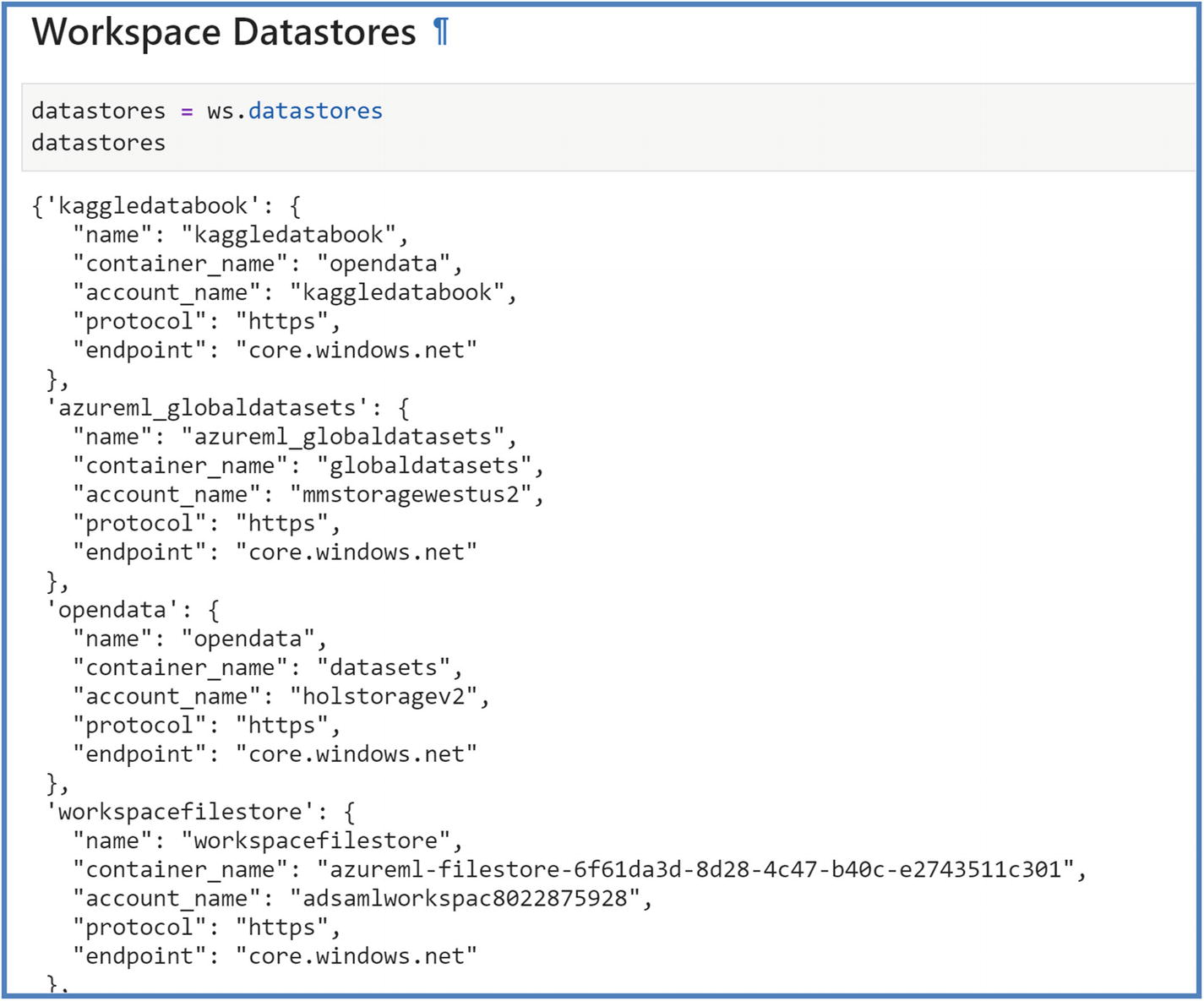 Figure 5-10
Azure ML workspace datastores
 Figure 5-11
Azure ML workspace default datastores
Register a new datastore. Figure 5-12
Azure ML registration of new datastores
- 6.Upload data to datastore to create a dataset or read existing data from datastore as a dataset. Dataset can be File or Tabular format; we will use Tabular Dataset as we are working with .csv. Run the next cells to upload data to Datastore and register the datasets in your workspace.
 Figure 5-13
Azure ML datasets
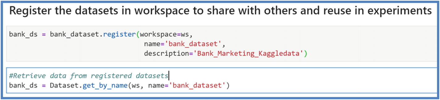 Figure 5-14
Azure ML datasets

Azure ML datasets studio view
Now that we have done logistics setup, let’s begin working on our specific use case in hand and build a machine learning model.
For this hands-on lab, we will use Kaggle dataset as a source as mentioned earlier and predict if a client will subscribe to term deposit. The term deposit can be defined as a cash investment held at a financial institution at an agreed rate of interest over an agreed period of time. The dataset includes some features like age, job, marital status, education, default, housing, and so on which we will study and use in our experiment.
Training on remote cluster
Directory/folder
Training script
Estimator
Model registration
- 1.Create a Directory/folder. A directory/folder is the key element of training as it contains all the necessary code, environment submitted from your development environment/local computer/compute instance to the remote cluster, in our case Azure ML compute cluster. Run the next cell to create a folder.
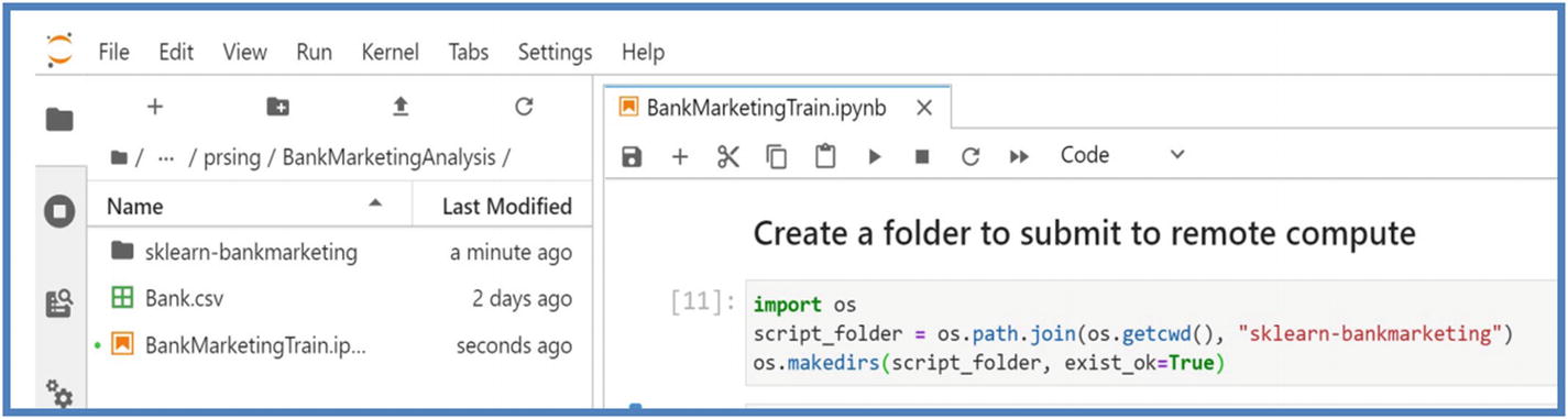 Figure 5-16
Azure ML workspace script folder
- 2.Create a Training Script. A training script contains all your code to train your model which gets submitted to Estimator class of experiment. This script should exist in the folder created in the last step. For bank marketing campaign, we will train XgBoost machine learning model which is a very common machine learning classifier and will predict the results of campaigning. In training script
- a.First, import all the necessary Python packages.
 Figure 5-17
Azure ML packages installation
- b.Pass the parameters using “argparse” library to train the machine learning model like it’s shown in the following. You can log parameters for each of your run to keep track of metrics and to reuse for future training of models. Here, we are logging parameters by using run.log() method.
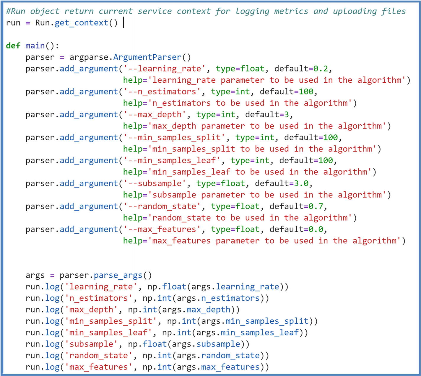 Figure 5-18
Experiment training script arguments
- c.
After passing parameters, you retrieve the input data for your experiment. The training script reads an argument to find the directory that contains data. We will use input data using data folder parameters and pass it in the script. We can use Dataset object to mount or download the files referred by it. Usually mounting is faster than downloading as mounting loads files at the time of processing and exists as mount point, that is, a reference to the file system.
- d.Next, users can combine Data Cleaning code and Model Training code, or they can create multiple experiments to keep track of these tasks individually. In this lab, we have combined both the tasks. Data Cleaning code includes changing the categorical values to numerical by using LabelEncoder or One Hot Encoding preprocessing SKlearn Python functions. Model Training code includes building the machine learning model, like for classification, we are using gradient boosting classifier. Other classifier/regressions methods can be used as well depending on the use case. The following is Data Cleaning code along with splitting it in train-test data.
 Figure 5-19
Experiment training script for cleaning
- e.Lastly, we would put XGB Classifier code and fit our model on training data using the parameters passed. The training script includes the code to save the model in to directory named output folder in your run. All the content of this directory gets uploaded to the workspace automatically. We will retrieve our model from this directory in the next steps. The following is the code we will use to fit the model on bank marketing training data. Run the create training script cell to save the train_bankmarketing.py in script folder.
 Figure 5-20
Experiment training script for model building and logging arguments
- 3.Create an Estimator. The estimator object is used to submit your run in the experiment. Azure ML includes pre-configured estimators for common machine learning frameworks like SKLearn, PyTorch, and generic estimators to be used for other frameworks. An estimator should include the following components to have successful run on remote compute:
- a.
Name of estimator object, like est or estimator.
- b.
Directory/folder that contains the code/scripts. All the content of this directory gets uploaded to the clusters for execution.
- c.
Script parameters if any.
- d.
The training script name, train_bankmarketing.py
- e.
Input Dataset for training as_named_input, training script will use this reference for data.
- f.
The compute target/remote compute. In our case, it’s Azure ML compute cluster named “ninjacpucluster.”
- g.
Environment definition for the experiment.
Run the next cells to create a SKLearn estimator and submit the experiment. Users can add tags at this time to keep tag with their experiments for easy reference.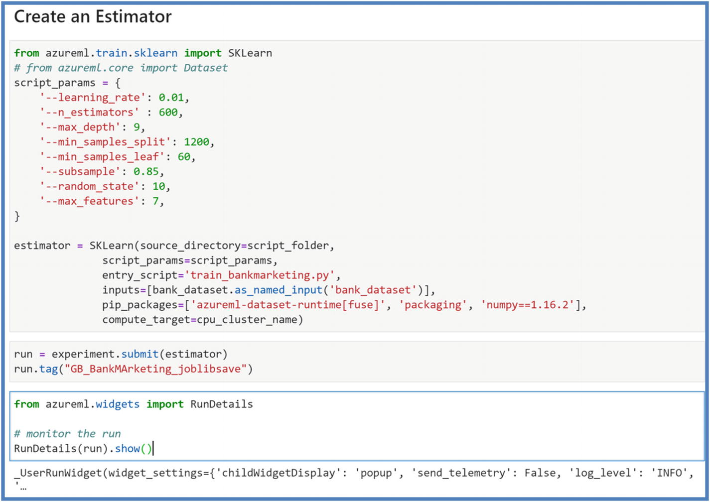 Figure 5-21
Azure ML experiment estimator
Once we submit the experiment, we can use RunDetails to check the progress. We can also click the link to check the progress on Azure ML workspace portal. Figure 5-22
Azure ML experiment run details
At this time, the following processes take place:The docker image is being created to develop Python environment specified in estimator. The first run takes longer than the subsequent runs as it’s creating a docker image with the dependencies defined. Unless dependencies are changed, the subsequent runs use the same docker image. The image is uploaded to the workspace and can be seen in logs.
Autoscaling happens if the remote cluster requires more nodes than available.
Running the entry script on compute target and datastore/datasets mounting for input data.
Preprocessing happens to copy the result of ./output directory of the run from VM of the cluster to the run history in your workspace.
Once the run finishes, we will be able to retrieve metrics logged in our experiment. This creates a testing environment for users to experiment/develop a good model and keep track of experiments. Once a satisfactory performance is achieved, users can go ahead and register the model. Use the following command to retrieve parameters, model performance, and so on.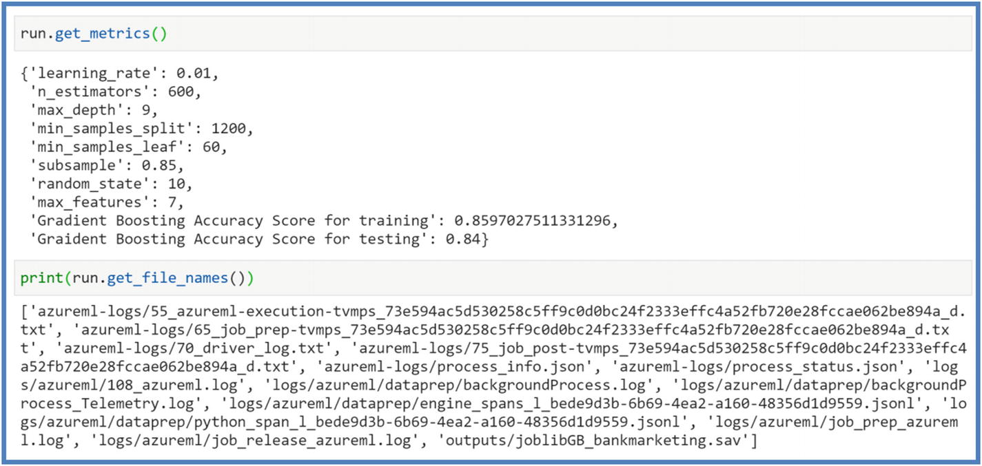 Figure 5-23
Azure ML experiment metrics
- 4.Register the model. This is the last step in Model Training life cycle. After running the experiment step, our model.pkl will exist in the run records of experiments in workspace. The model registry contains your trained models and is accessible to other users in workspace. Once the model is registered with version number, later it can be used to query, examine, deploy, and for MLOps purposes (refer to Chapter8). Run the next cell to register the model.
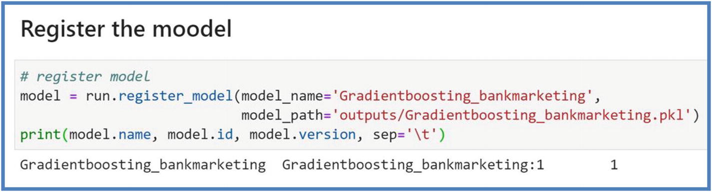 Figure 5-24
Azure ML model registration
The model can come from Azure ML or from somewhere else. While registering the model, the path of either a cloud location or local directory is provided. The path is used to locate the model files to upload as a registration process.
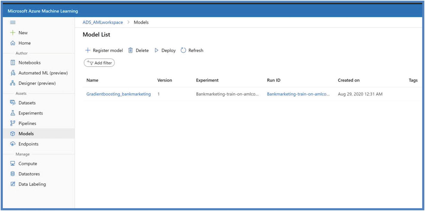
Azure ML model on studio portal
Deploying your model as web service
Deploying your model as a web service simply means creating a docker image that captures machine learning model, scoring logic, and its authentication parameters. We will now go ahead and deploy our model on Azure container instance (ACI) . Container instance runs docker containers on-demand in a managed, serverless Azure environment. It’s an easy solution to test the deployment performance, scoring workflow, and debug issues. Once the deploy model workflow is built, we would deploy the model to Azure Kubernetes Service for more scalable production environment. Refer to Chapter 4 to understand the suitable service for deployments.
Scoring script to understand the model workflow and run the model to return the prediction
Configuration file to define the environment/software dependencies needed for deployment
Deployment configuration to define characteristics of compute target to host the model and scoring script
- 1.Create Scoring Script. This script is specific to your model and should incorporate data format/schema expected by the model. The script will receive the data submitted to the web service, pass it to the registered model, and return the response/predictions. Scoring Script requires two functions:
- a.
Init(): This function is called when the service is initialized and loads your model in a global object.
- b.
Run(rawdata): This function is called when the new data is submitted and uses the model loaded in init() function to make the predictions.
Run the next cell to create the scoring script for our use case. Figure 5-26
Azure ML scoring script
- 2.Configuration File. This file includes model’s runtime environment in Environment object and CondaDependencies needed by your model. Make sure to pass specific versions of Python libraries used while training the model. Run the next cell to create configuration file.
 Figure 5-27
Azure ML environment configuration file
- 3.Deployment Configuration. This configuration is required to create the docker image specific to the compute target. We will be deploying our model to Azure container instance (ACI) first for testing purposes. Run the following code to deploy your model to ACI. This process will take 5–10 minutes or longer depending on model trained and software dependencies.
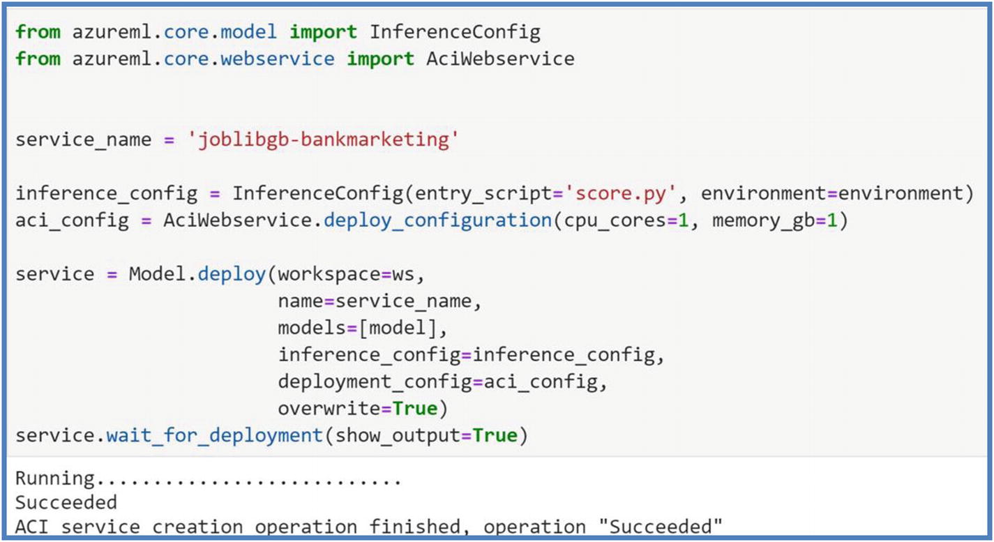 Figure 5-28
Azure ML deployment configuration on Azure container instance
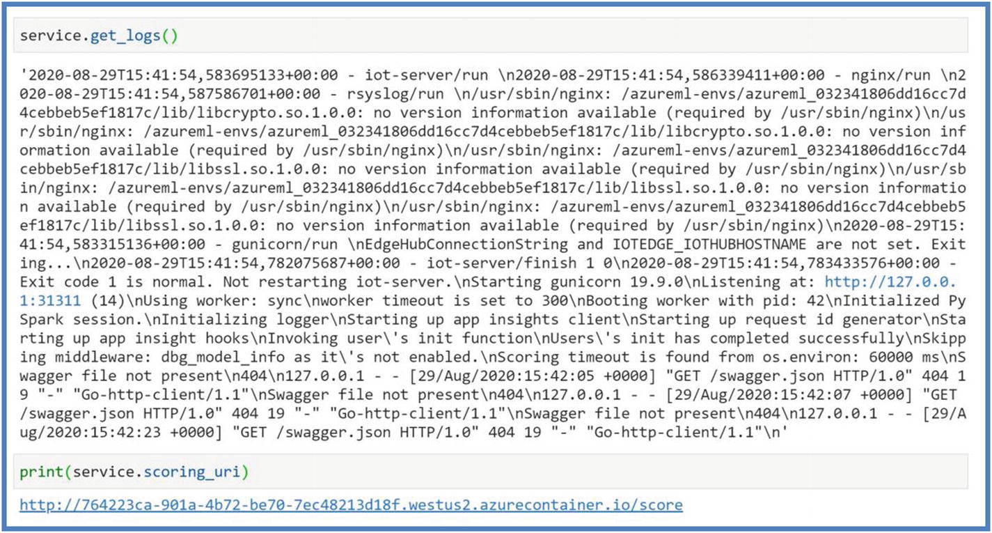 Figure 5-29
Azure ML deploy logs
If deployment fails for multiple reasons, use commands shown in Figure 5-29 to get the logs for troubleshooting purposes. Once the service deployment is succeeded, we will be able to retrieve our scoring URL using the service.scoring_uri shown in Figure 5-29 .

Azure ML deployed model web service test
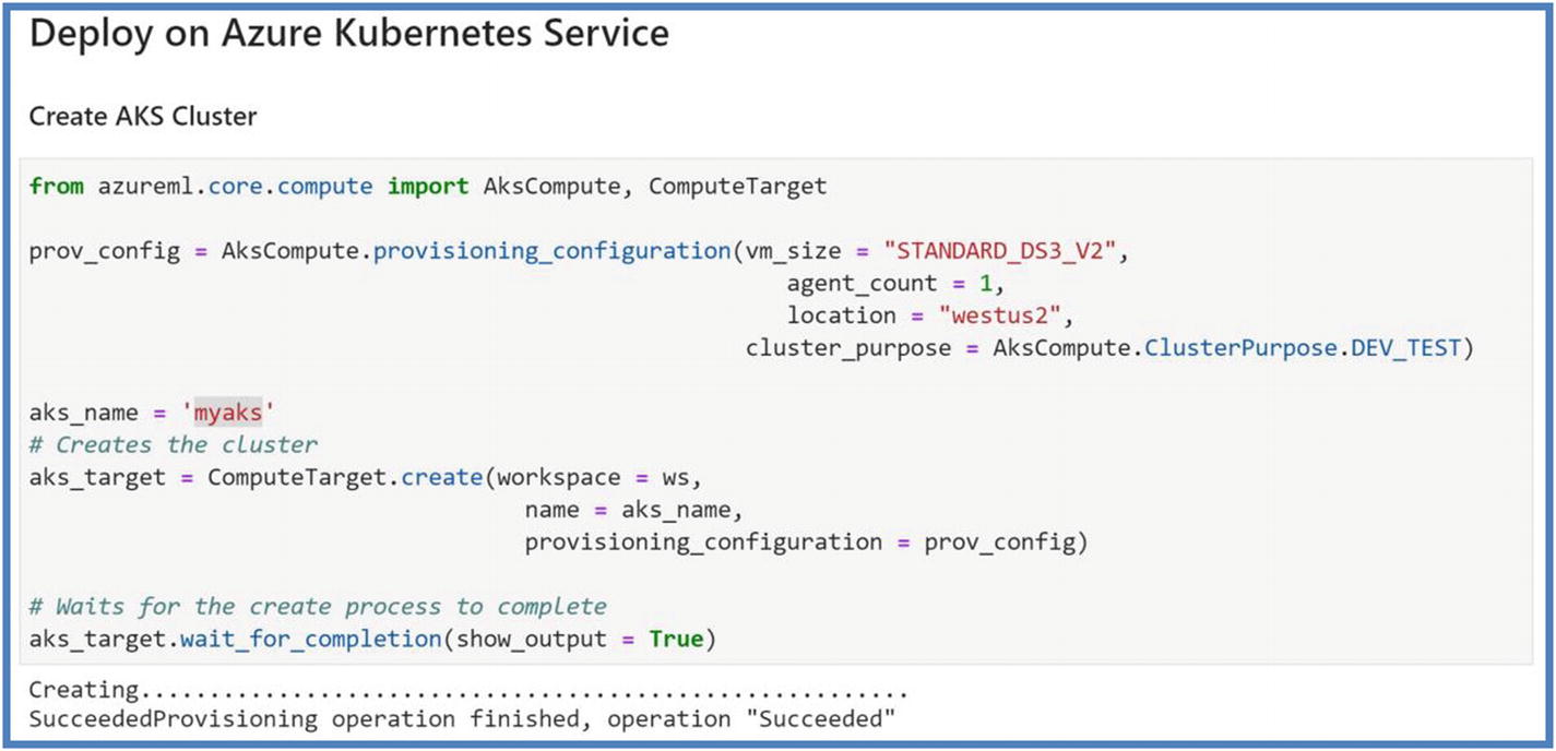
Azure Kubernetes cluster creation
Users can attach the existing AKS cluster as well. While creating or attaching, cluster_purpose defines the minimum virtual CPUs/GPUs required. For cluster_purpose = Dev_Test, at least 2 virtual CPUs are recommended; for cluster_purpose = Fast_PROD, at least 12 virtual CPUs are recommended.

Azure ML deployment configuration on Azure Kubernetes Service

Azure ML deployed models as web services
Automated Machine Learning (AutoML)
Automated Machine Learning is a technique to design probabilistic machine learning models to automate experimental decisions while building models and optimizing performance. It allows users to try multiple algorithms, their hyperparameters tuning, and preprocessing transformations on your data combined with scalable cloud-based compute offerings. The automated process of finding the best performing model based on primary metric saves huge amount of time spent in manual trial and error processes. The goal of introducing AutoML is to accelerate and simplify artificial intelligence processes for a wider audience including data scientists, data engineers, business users, and developers. With AutoML, data scientists can automate part of their workflow and focus on other more important aspects of business objectives, while business users who don’t have advanced data science and machine learning/coding expertise can benefit from AutoML user interface and build out models in minutes.
- 1.Identify ML problem:
- a.
Classification
- b.
Regression
- c.
Forecasting
- 2.
Python Azure ML SDK or Azure ML Studio: AutoML studio is available only in enterprise edition. The following is a comparison of features supported in both.
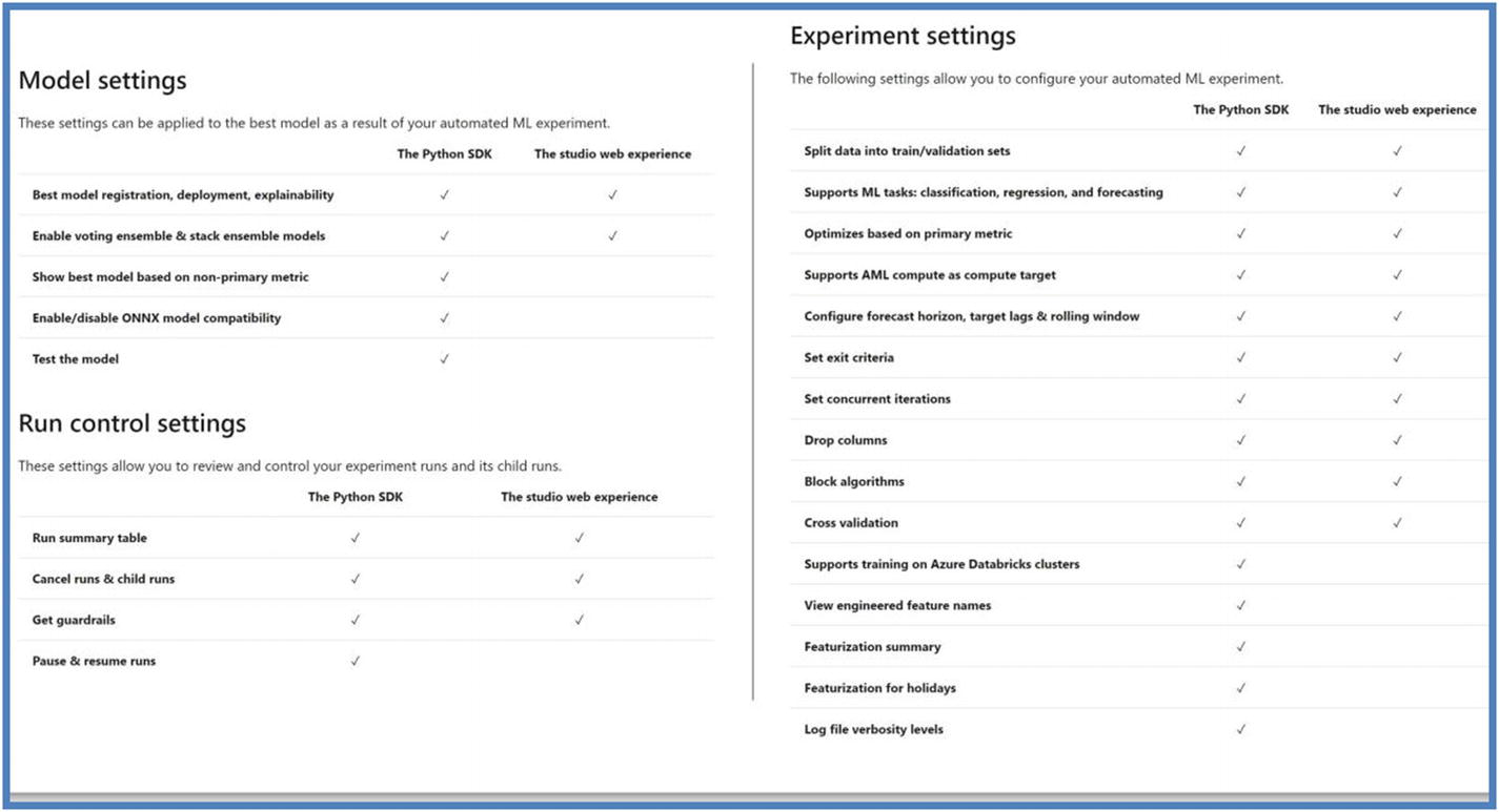
Azure ML Studio vs. Azure ML SDK features. Source: https://docs.microsoft.com/en-us/azure/machine-learning/concept-automated-ml#parity
For purposes of hands-on lab on AutoML, we will use the same bank marketing dataset and develop a classification model to predict the term deposit using both web and Python SDK. So let’s go ahead and build our experiment using AutoML studio web experience and Python SDK.
AutoML studio web
- 1.Click the new Automated ML run as shown in Figure 5-35.
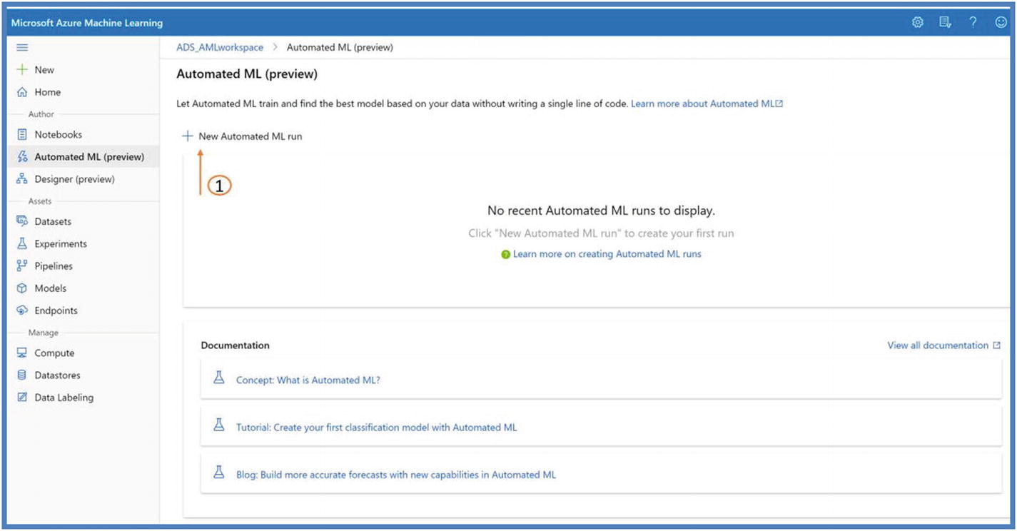 Figure 5-35
AutoML on Azure ML Studio
- 2.Next, we will use the Dataset created earlier. Users can also create a new dataset at this point from the following available options.
 Figure 5-36
AutoML experiment
A good use case will be to include open dataset like weather or census. Azure ML offers a variety of open datasets.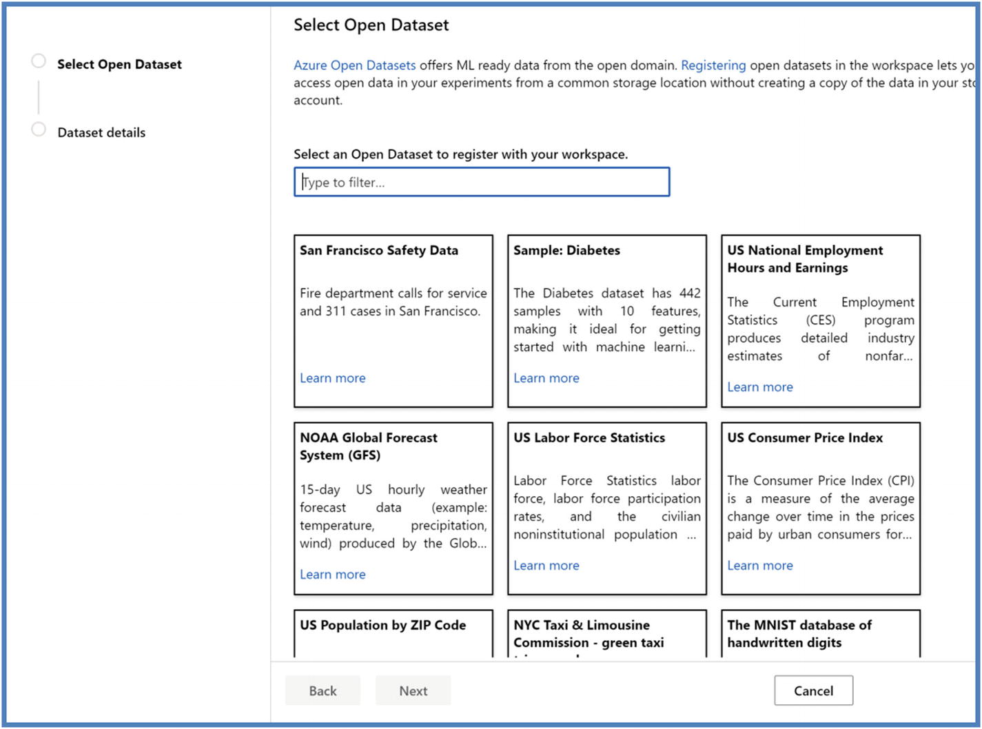 Figure 5-37
Azure open datasets
We will use bank dataset created previously (in this chapter) and will do a quick preview by clicking preview tab. Click Next after done previewing to continue with AutoML experiment.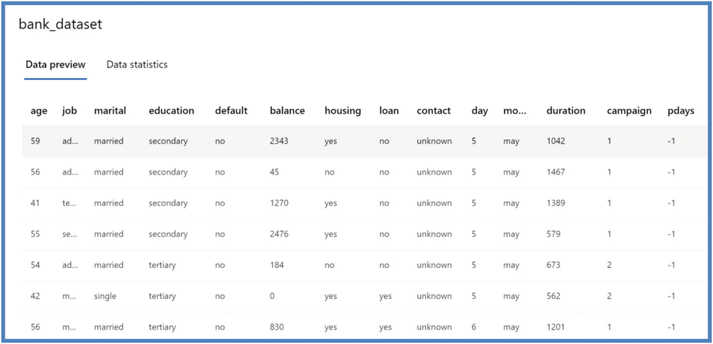 Figure 5-38
AutoML data preview
- 3.Next, we will configure Experiment settings. Click Next.
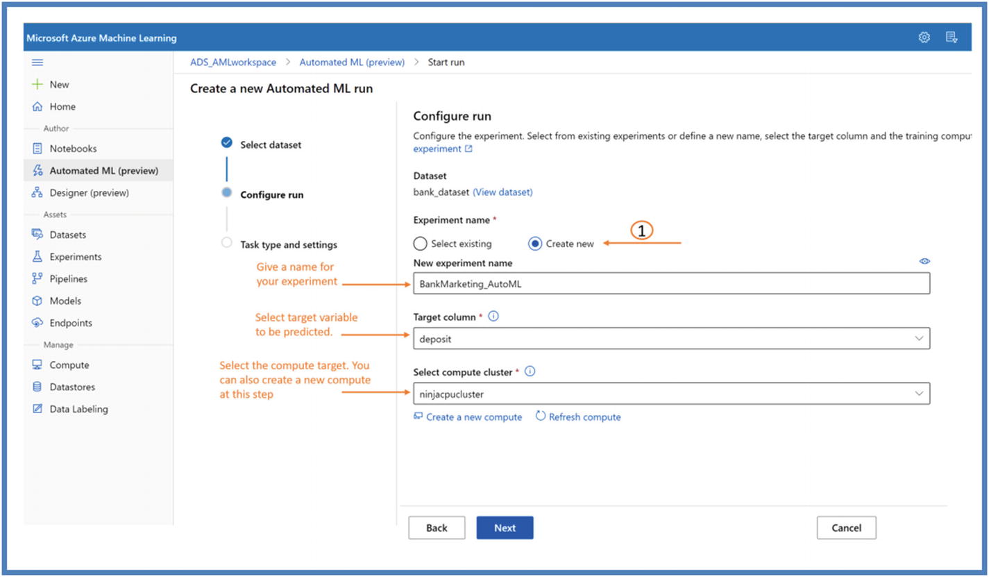 Figure 5-39
AutoML experiment configure
- 4.At this step, we will pick classification for our use case. Users can enable deep learning option as well to incorporate deep learning models in machine learning algorithms, but it will take more time to finish the experiment.
 Figure 5-40
AutoML task identification

AutoML additional configuration settings
Users can also control additional features here. We will check off pdays at this point (shown in Figure 5-42) and click Save.

AutoML additional featurization settings
AutoML experiment run details

AutoML models
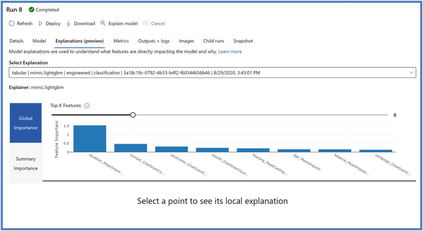
AutoML feature explanations
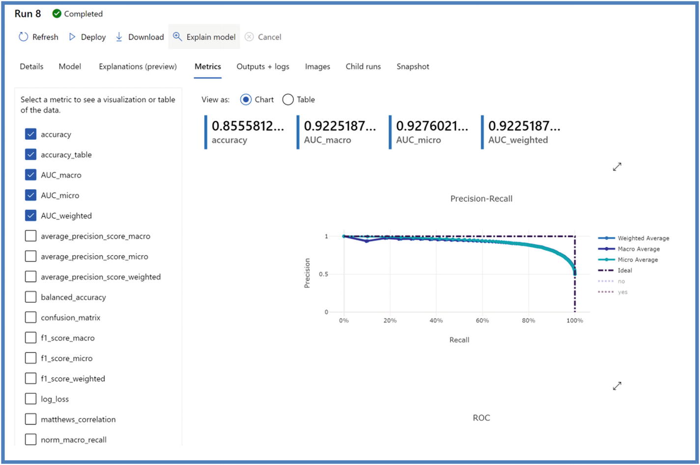
AutoML metrics results

AutoML model deployment on studio portal
Next, we will deploy the model. Users can deploy the model on either ACI or AKS from the portal itself by first selecting the model and clicking Deploy (shown in Figure 5-47).
AutoML Python SDK
From all the previous datastore/dataset setup, we will go ahead and start writing code in JupyterLab to create an AutoML experiment in Python SDK.
This hands-on lab will use previous prerequisite setup. If you’ve not run Azure ML SDK lab and doing AutoML lab, please run through the prerequisite setup section before starting this lab.
AutoML Python SDK setup
- 1.
Create a Jupyter notebook and put the code shown in Figure 5-48. To follow along with the code, users can also Git clone the repository from GitHub. To do that, refer to the following location. We will be using Automl_bankmarketing.ipynb notebook for the code.
https://github.com/singh-soh/AzureDataScience/tree/master/Chapter05_AzureML_Part2
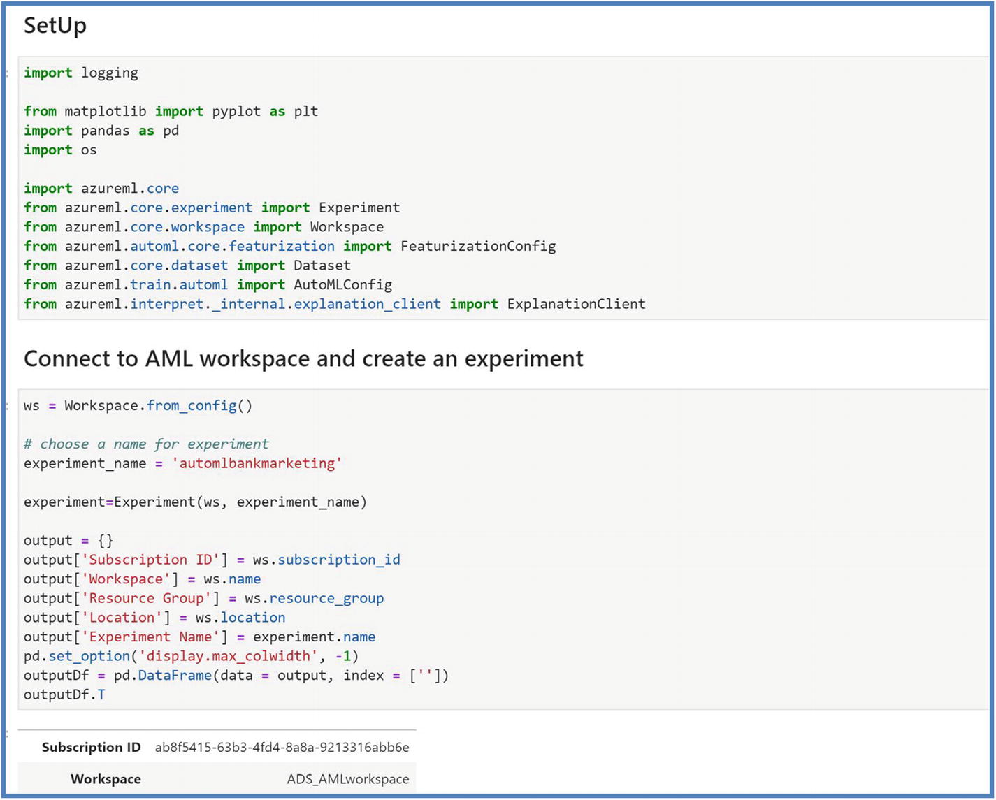
- 2.
Run the cells to set up with libraries and connect to Azure ML workspace and instantiate an experiment.
- 3.Run the next cell to create a new/or use a previously created compute target. We will use previously created “ninjacpucluster” to create AutoML experiment (shown in Figure 5-49).
 Figure 5-49
AutoML Python SDK compute cluster
- 4.Next, let’s load the data from previously created ‘bank_Dataset’. We will also split data into training and testing at this point.
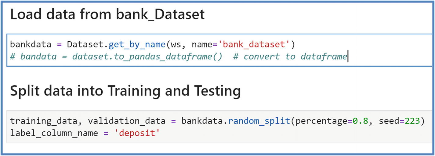 Figure 5-50
AutoML Python SDK dataset and train/test split
- 5.Next, we will configure AutoML settings. These settings define how your AutoML experiment will be run on what compute. Run the next cell to configure these settings.
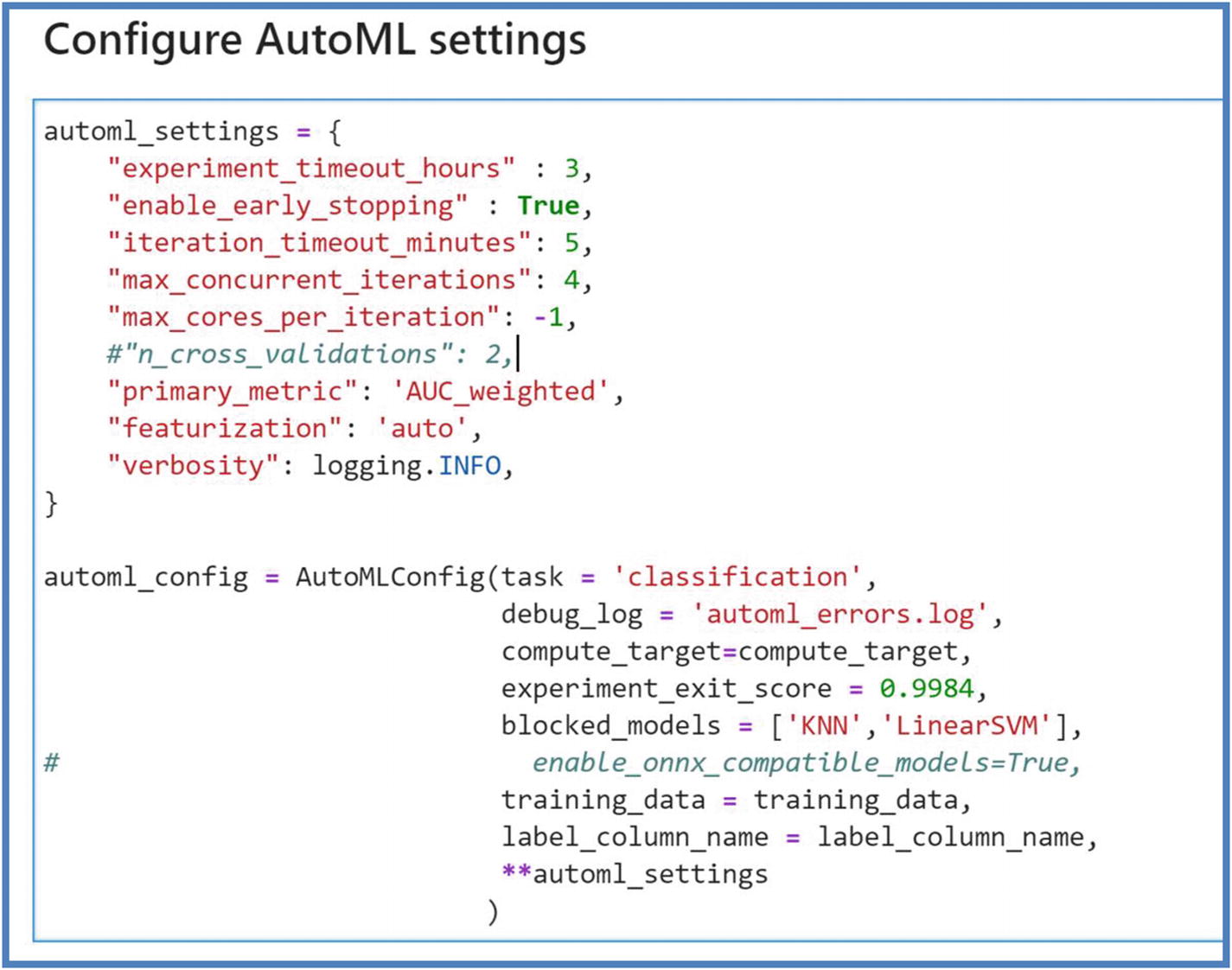 Figure 5-51
AutoML Python SDK configuration settings
The following is a short list of settings users can configure while running the experiment in Python SDK. For complete list, refer to detailed explanation here: https://docs.microsoft.com/en-us/python/api/azureml-train-automl-client/azureml.train.automl.automlconfig.automlconfig?view=azure-ml-py- a.
task: Regression or classification or forecasting.
- b.
compute_target: Remote cluster/machine this experiment will use to create the run.
- c.
Primary_metric: Models are optimized based on this metric.
- d.
Experiment_exit_score: Value indicating the target of primary metric.
- e.
Blocked_models: User-specified models that will be ignored in training.
- f.
Training_data: Input dataset including features and label column.
- g.
Label_column_name: Target variable that needs to be predicted.
- h.
Experiment_timeout_hours: Maximum amount of time an experiment can take to terminate all the iterations.
- i.
Enable_early_stopping : Flag to enable early termination if the score is not improving in the iterations short term.
- j.
Iteration_timeout_minutes: Maximum time in minutes that each iteration can run before it terminates. Here, an iteration is total number of different algorithms and parameter combinations to test for AutoML experiment.
- k.
Max_concurrent_iterations: Maximum iterations executed in parallel.
- l.
Max_cores_per_iteration: Maximum number of threads to use for an iteration.
- m.
Featurization: Auto or off to determine if featurization should be done automatically or not or if customized featurization will be used.
- 6.After Autol config settings, we would go ahead and submit the experiment to find the best-fitted model for our bank marketing prediction. You can track this experiment by following the link to Azure ML portal workspace; it will take 15–20 minutes to finish running. Run the next cell to submit the experiment.
 Figure 5-52
AutoML Python SDK experiment
- 7.Once it’s completed, we will be able to retrieve the best-fitted model by following this command.
 Figure 5-53
AutoML Python SDK best-fitted model retrieved
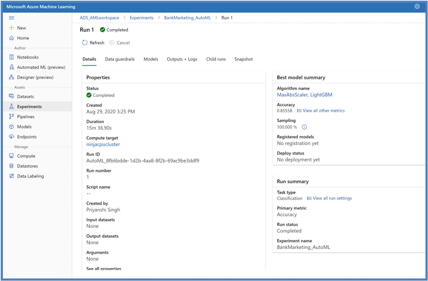
- 8.We will be able to see the finished run on the portal as well along with best model trained considering the primary metric defined.
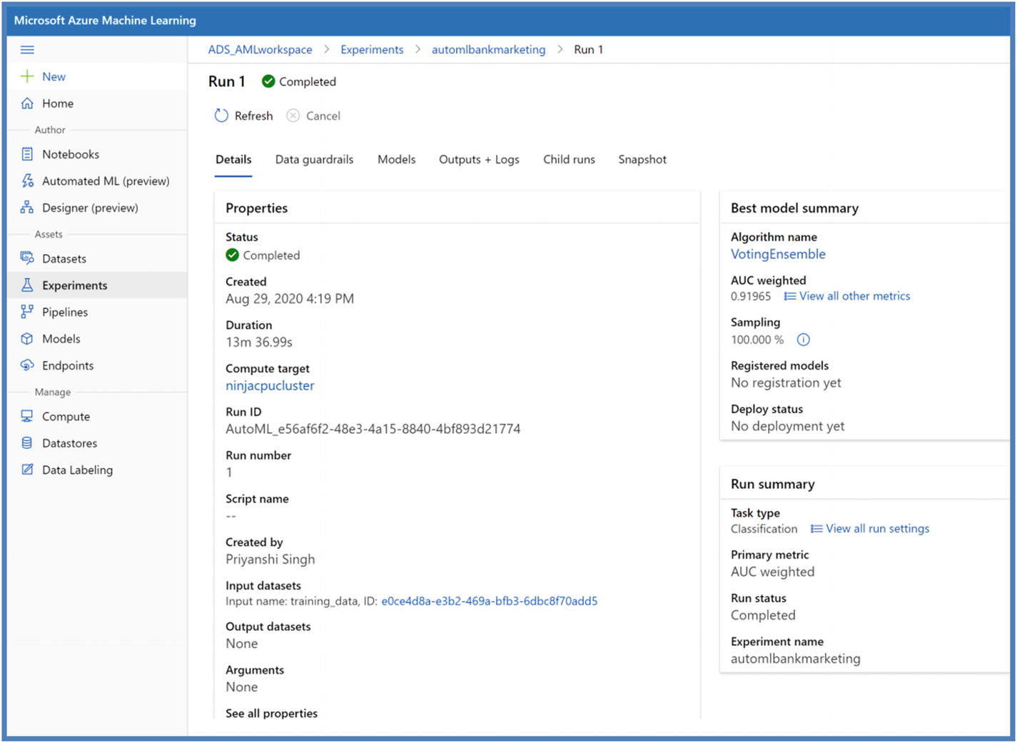 Figure 5-54
AutoML Python SDK model on studio portal
The resulting model is different in both the methods – AutoML on portal and AutoML on Python SDK. This is primarily due to the different primary metric used along with different configurations. However, users can always look into the metrics score by clicking “View all other metrics.”
- 9.Next step will be to register the best-fitted model and deploy it. These steps are the same as Azure ML Python SDK experiment done before; refer to the same code to deploy this model. To register the model, run the next command.
 Figure 5-55
AutoML Python SDK model registration
Summary
In this chapter, we were able to do hands-on using Azure ML Python SDK with bank marketing dataset, logging metrics, model versions, and how to deploy the model to Azure container instance (ACI) and Azure Kubernetes Service (AKS). We also learned Automated Machine Learning (AutoML) using portal as well as Python SDK. There are several use cases for which Azure Machine Learning can be used. This chapter gives users a good understanding and hands-on experience to Azure ML, and users are encouraged to keep learning and explore ways to leverage ML on Azure whether on local computer or Azure Databricks workspace or Azure ML compute instance or a data science virtual machine. Please refer to this repo for plenty of resources and material to keep learning: https://github.com/singh-soh/AzureDataScience/tree/master/Chapter05_AzureML_Part2. To manage ML production life cycle, we will learn about Azure ML pipelines and ML operations in Chapter 8 and understand how to automate the workflows and follow Continuous Integration/Continuous Delivery (CI/CD) principles.