
Chapter 7
Trees
CHAPTER OUTLINE
7.1 INTRODUCTION
There are situations where the nature of data is specific and cannot be represented by linear or sequential data structures. For example, as shown in Figure 7.1 hierarchical data such as ‘types of computers’ is non-linear by nature.
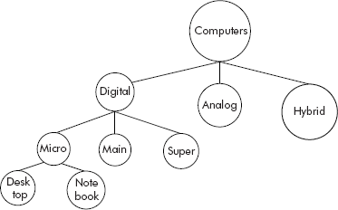
Fig. 7.1 Hierarchical data
Situations such as roles performed by an entity, options available for performing a task, parent–child relationships demand non-linear representation. A tourist can go from Mumbai to Goa by any of the options shown in Figure 7.2.
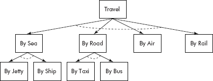
Fig. 7.2 Options available for travelling from Mumbai to Goa
Similarly, the information about folders and files is kept by an operating system as a set of hierarchical nodes as shown in Figure 7.3.
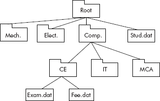
Fig. 7.3 The representation of files and folders
Even the phrase structure of a sentence of a language is represented in a similar fashion (see Figure 7.4).
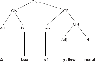
Fig. 7.4 The phrase structure of a sentence
A critical look at the data representations, shown in Figures 7.1–7.4, indicates that the structures are simply upside down trees where the entity at the highest level represents the root and the other entities at lower level are themselves roots for sub-trees. For example in Figure 7.2, the entity ‘Travel’ is the root of the tree and the options ‘By Sea’ and ‘By Road’, ‘By Air’ and ‘By Rail’ are called child nodes of ‘Travel’, the root node. It may be noted that the entities ‘By Road’, ‘By Air’ are themselves roots of sub- trees. The nodes which do not have child nodes are called leaf nodes. For example, the nodes such as ‘By Jetty’, ‘By Ship’, ‘By Air’, etc. are leaf nodes.
A tree can be precisely defined as a set of 1 or more nodes arranged in a hierarchical fashion. The node at the highest level is called a root node. The other nodes are grouped into T1; T2…Tk subsets. Each subset itself is a tree. A tree with zero nodes is called an empty tree.
It may be noted that the definition of a tree is a recursive definition, i.e., the tree has been defined in its own terms. The concept can be better understood by the illustration given in Figure 7.5.
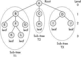
Fig. 7.5 The tree and its related terms
From Figure 7.5, the following components of a tree can be identified
| Root | : A |
| Child nodes of A | : B, C, D |
| Sub-Trees of A | : T1, T2, T3 |
| Root of T1 | : B |
| Root of T2 | : C |
| Root of T3 | : D |
| Leaf nodes | : E, G, H, I, J, K, L |
Before proceeding to discuss more on trees, let us have a look at basic terminology used in context of trees as given in Section 7.2.
7.2 BASIC TERMINOLOGY
Parent: An immediate predecessor of a node is called its parent.
Example: D is parent of I and J.
Child: The successor of a node is called its child.
Example: I and J are child nodes of node D.
Sibling: Children of the same parent are called siblings.
Example: B, C, and D are siblings. E, F, and G are also siblings.
Leaf: The node which has no children is called a leaf or terminal node.
Example: I, J, K, L, etc. are leaf nodes.
Internal node: Nodes other than root and leaf nodes are called internal nodes or non-terminal nodes.
Example: B, C, D and F are internal nodes.
Root: The node which has no parent.
Example: A is root of the tree given in Figure 7.5.
Edge: A line from a parent to its child is called an edge.
Example: A-B, A-C, F-K are edges.
Path: It is a list of unique successive nodes connected by edges.
Example: A-B-F-L and B-F-K are paths.
Depth: The depth of a node is the length of its path from root node. The depth of root node is taken as zero.
Example: The depths of nodes G and L are 2 and 3, respectively.
Height: The number of nodes present in the longest path of the tree from root to a leaf node is called the height of the tree. This will contain maximum number of nodes. In fact, it can also be computed as one more than the maximum level of the tree.
Example: One of the longest paths in the tree shown in Figure 7.3 is A-B-F-K. Therefore, the height of the tree is 4.
Degree: Degree of a node is defined as the number of children present in a node. Degree of a tree is defined equal to the degree of a node with maximum children.
Example: Degree of nodes C and D are 1 and 2, respectively. Degree of tree is 3 as there are two nodes A and B having maximum degree equal to 3.
It may be noted that the node of a tree can have any number of child nodes, i.e., branches. In the same tree, any other node may not have any child at all. Now the problem is how to represent such a general tree where the number of branches varies from zero to any possible number. Or is it possible to put a restriction on number of children and still manage this important non-linear data structure? The answer is ‘Yes’. We can restrict the number of child nodes to less than or equal to 2. Such a tree is called binary tree. In fact, a general tree can be represented as a binary tree and this solves most of the problems. A detailed discussion on binary trees is given in next section.
7.3 BINARY TREES
Binary tree is a special tree. The maximum degree of this tree is 2. Precisely, in a binary tree, each node can have no more than two children. A non-empty binary tree consists of the following:
- A node called the root node
- A left sub-tree
- A right sub-tree
Both the sub-trees are themselves binary trees as shown in Figure 7.6.
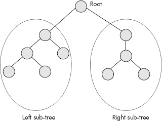
Fig. 7.6 A binary tree
Kindly note that contrary to a general tree, an empty binary tree can be empty, i.e., may have no node at all. Examples of valid binary trees are given in Figure 7.7.
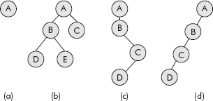
Fig. 7.7 Examples of valid binary trees
Since the binary trees shown in Figure 7.7 are not connected by a root, it is called a collection of disjoint trees or a forest. The binary tree shown in Figure 7.7 (d) is peculiar tree in which there is no right child. Such a tree is called skewed to the left tree. Similarly, there can be a tree skewed to the right, i.e., having no left child.
There can be following two special cases of binary tree:
- Full binary tree
- Complete binary tree
A full binary tree contains the maximum allowed number of nodes at all levels. This means that each node has exactly zero or two children. The leaf nodes at the last level will have zero children and the other non-leaf nodes will have exactly two children as shown in Figure 7.8.
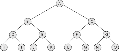
Fig. 7.8 A full binary tree
A complete binary tree is a full tree except at the last level where all nodes must appear as far left as possible. A complete binary tree is shown in Figure 7.9. The nodes have been numbered and there is no missing number till the last node, i.e., node number 12.
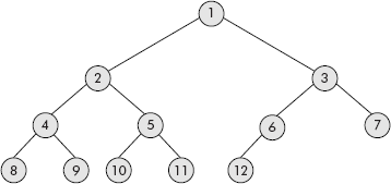
Fig. 7.9 Complete binary tree
Consider the binary tree given in Figure 7.10 which violates the condition of the complete binary tree as the node number 11 is missing. Therefore, it is not a complete binary tree because there is a missing intermediate node before the last node, i.e., node number 12.
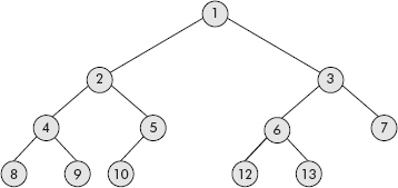
Fig. 7.10 An incomplete binary tree
7.3.1 Properties of Binary Trees
The binary tree is a special tree with degree 2. Therefore, it has some specific properties which must be considered by the students before implementing binary trees; these are:
Consider the binary tree given in Figure 7.10.
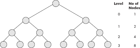
Fig. 7.10 A full binary tree
- The maximum number of nodes at level 0 = 1
The maximum number of nodes at level 1 = 2
The maximum number of nodes at level 2 = 4
The maximum number of nodes at level 3 = 8
By induction, it can be deduced that maximum nodes in a binary tree at level I = 2I
- The maximum number of nodes possible in a binary tree of depth 0 = 1
The maximum number of nodes possible in a binary tree of depth 1 = 3
The maximum number of nodes possible in a binary tree of depth 2 = 7
The maximum number of nodes possible in a binary tree of depth 3 = 15
By induction, it can be deduced that maximum nodes in a binary tree at depth k = 2k − 1
- It may be noted that the number of leaf nodes is 1 more than the number of non-leaf nodes in a non-empty binary tree. For example, a binary tree of depth 2 has 4 leaf nodes and 3 non-leaf nodes. Similarly, for a binary tree of depth 3, number of leaf nodes is 8 and non-leaf nodes is 7.
- Similarly, it can be observed that the number of nodes is 1 more than the number of edges in a non-empty binary tree, i.e., n = e + 1, where n is number of nodes and e is number of edges.
- A skewed tree contains minimum number of nodes in a binary tree. Consider the skewed tree given in Figure 7.7 (d). The depth of this tree is 3 and the number of nodes in this tree is equal to 4, i.e., 1 more than the depth. Therefore, it can be observed that the number of nodes in a skewed binary tree of a depth k is equal to k + 1. In other words, it can be said that minimum number of nodes possible in a binary tree of depth k is equal to k + 1.
7.4 REPRESENTATION OF A BINARY TREE
The binary tree can be represented in two ways—linear representation and linked representation. A detailed discussion on both the representations is given in subsequent sections.
7.4.1 Linear Representation of a Binary Tree
A binary tree can be represented in a one-dimensional array. Since an array is a linear data structure, the representation is accordingly called linear representation of a binary tree. In fact, a binary tree of height h can be stored in an array of size 2h − 1. The representation is quite simple and follows the following rules:
- Store a node at ith location of the array.
- Store its left child at (2*i)th location.
- Store its right child at (2*i + 1)th location.
- The root of the node is always stored at first location of the array.
Consider the tree given in Figure 7.8. Its linear representation using an array called linTree is given in Figure 7.11.
In an array of size N, for the given node i, the following relationships are valid in linear representation:
- leftChild (i) = 2*i { When 2*i > N then there is no left child }
- rightChild(i) = 2*i + 1 { When 2*i +1 > N then there is no right child }
- parent (i) = [i/2] { node 0 has no parent – it is a root node }
The following examples can be verified from the tree shown in Figure 7.8:
- The parent of node at i = 5 (i.e., E) would be at [5/2] = 2, i.e., B.
- The left child of node at i = 4 (i.e., D) would be at (2*4) = 8, i.e., H.
- The right child of node i = 10 (i.e., J) would be at (2*10) + 1 = 21 which is > 15, indicating that it has no right child.
It may be noted that this representation is memory efficient only when the binary tree is full whereas in case of skewed trees, this representation is very poor in terms of wastage of memory locations. For instance, consider the skewed tree given in Figure 7.7 (d). Its linear representation using an array called skewTree is given in Figure 7.12.
It may be noted that out of 15 locations, only 4 locations are being used and 11 are unused resulting in almost 300 per cent wastage of storage space.
The disadvantages of linear representation of binary tree are as follows:
- In a skewed or scanty tree, a lot of memory space is wasted.
- When binary tree is full then space utilization is complete but insertion and deletion of nodes becomes a cumbersome process.
- In case of a full binary tree, insertion of a new node is not possible because an array is a static allocation and its size cannot be increased at run time.
7.4.2 Linked Representation of a Binary Tree
A critical look at the organization of a non-empty binary tree suggests that it is a collection of nodes. Each node comprises the following:
- It contains some information.
- It has an edge to a left child node.
- It has an edge to a right child node.
The above components of a node can be comfortably represented by a self-referential structure consisting of DATA part, a pointer to its left child (say leftChild), and a pointer to its right child (say rightChild) as shown in Figure 7.13.
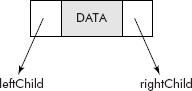
Fig. 7.13 A node of a binary tree
Now the node shown in Figure 7.13 will become the building block for construction of a binary tree as shown in Figure 7.14.
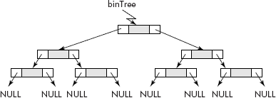
Fig. 7.14 A binary tree represented through linked structures
It may be noted that the root node is pointed by a pointer called binTree. Both leftChild and rightChild of leaf nodes are pointing to NULL. Let us now try to create binary tree.
Note: Most of the books create only binary search trees which are very specific trees and easy to build. In this book a novel algorithm is provided that creates a generalized binary tree with the help of a stack. The generalized binary tree would be constructed and implemented in ‘C’ so that the reader gets the benefit of learning the technique for building binary trees.
7.4.2.1 Creation of a Generalized Binary Tree
Let us try to create the tree shown in Figure 7.15.
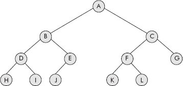
Fig. 7.15 The binary tree to be created
A close look at the tree shown in Figure 7.15 gives a clue that any binary tree can be represented as a list of nodes. The list can be prepared by following steps:
- Write the root.
- Write its sub-trees within a set of parenthesis, separated by a comma.
- Repeat steps 1 and 2 for sub-trees till you reach leaf nodes. A missing child in a non-leaf node is represented as $.
By applying the above steps on binary tree of Figure 7.15, we get the following list:
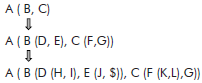
So the final list is: A ( B (D (H, I), E (J, $)), C (F (K,L),G))
Now the above list can be used to create its originating binary tree with the help of a stack. It is stored in a list called treeList as given below:
treeList[] = {’A’, ’(’, ’B’, ’(’, ’D’,’(’,’H’, ’I’,’)’, ’E’,’(’, ’J’,’$’, ’)’,’)’,’C’,’(’,’F’,’(’,’K’,’L’,’)’,’G’,’)’,’)’,’#’};
The algorithm that uses the treeList and a stack to create the required binary tree is given below:
Algorithm createBinTree()
{
  Step
  1. Take an element from treeList;
  2. If (element != ’(’ && element != ’)’ && element != ’$’  && element !=’#’)
  {
   Take a new node in ptr;
   DATA(ptr) = element;
   leftChild (ptr) = NULL;
   rightChild (ptr) = NULL;
   Push (ptr);
  }
  3. if (element = ’)’ )
  {
   Pop (LChild);
   Pop (RChild);
   Pop(Parent);
   leftChild(Parent) = LChild;
   rightChild(Parent) = RChild;
   Push (Parent);
  }
  4. if (element = ’(’ ) do nothing;
  5. if (element = ’$’ ) Push (NULL);
  6. repeat steps 1 to 5 till element != #;
  7. Pop (binTree);
  8. stop.
}
A simulation of the above algorithm for the following treeList is given in Figure 7.16.
treeList[] = {’A’, ’(’, ’B’, ’(’, ’D’,’(’,’H’, ’I’,’)’, ’E’,’(’, ’J’,’$’, ’)’,’)’,’C’,’(’,’F’,’(’,’K’,’L’,’)’,’G’,’)’,’)’,’#’};
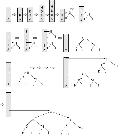
Fig. 7.16 The creation of binary tree using the algorithm createBinTree()
It may be noted that the algorithm developed by us has created exactly the same tree which is shown in Figure 7.15.
7.4.3 Traversal of Binary Trees
A binary tree is traversed for many purposes such as for searching a particular node, for processing some or all nodes of the tree and the like. A system programmer may implement a symbol table as binary search tree and process it in a search/insert fashion.
The following operations are possible on a node of a binary tree:
- Process the visited node – V.
- Visit its left child – L.
- Visit its right child – R.
The travel of the tree can be done in any combination of the above given operations. If we restrict ourselves with the condition that left child node would be visited before right child node, then the following three combinations are possible:
- L-V-R : Inorder travel
- travel the left sub-tree
- process the visited node
- travel the right sub-tree
- V-L-R : Preorder travel
- process the visited node
- travel the left sub-tree
- travel the right sub-tree
- L-R-V : Postorder travel
- travel the left sub-tree
- travel the right sub-tree
- process the visited node
It may be noted that the travel strategies given above have been named as preorder, inoder, and postorder according to the placement of operation: ‘V’ –’process the visited node’. Inorder (L-V-R) travel has the operation ‘V’ in between the other two operations. In preorder (V-L-R), the operation ‘V’ precedes the other two operations. Similarly, the postorder traversal has the operation ‘V’ after the other two operations.
7.4.3.1 Inorder Travel (L-V-R)
This order of travel, i.e., L-V-R requires that while travelling the binary tree, the left sub-tree of a node be travelled first before the data of the visited node is processed. Thereafter, its right sub-tree is travelled.
Consider the binary tree given in Figure 7.17. Its root node is pointed by a pointer called Tree.
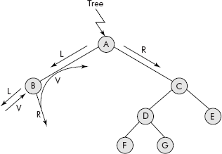
Fig. 7.17 Partial travel of L-V-R order
The travel starts from root node A and its data is not processed as it has a left child which needs to be travelled first indicated by the operation L. Therefore, we move to B. As B has no left child, its data is processed indicated by the operation V. Now the right child of B needs to be travelled which is NULL, indicated by the operation R. Thus, the travel of B is complete and the travel of left sub-tree of A is also over. As per the strategy, the data of A is processed (V) and the travel moves to its right sub-tree, i.e., to node C (R). The process is repeated for this sub-tree with root node as C. The final trace of the travel is given below:
B A F D G C E
An algorithm for inorder travel (L-V-R) is given below. It is provided with the pointer called Tree that points to the root of the binary tree.
   Algorithm inorderTravel(Tree)
   {
     if (Tree == NULL) return
     else
     {
      inorderTravel (leftChild (Tree));
      process DATA (Tree);
      inorderTravel (rightChild (Tree));
     }
   }
Example 1: Write a program that creates a generalized binary tree and travels it using an inorder strategy. While travelling, it should print the data of the visited node.
Solution: We would use the algorithms createBinTree() and inorderTravel(Tree) to write the program.
The required program is given below:
   /* This program creates a binary tree and travels it using inorder fashion */

   #include <stdio.h>
   #include <alloc.h>
   #include <conio.h>

   struct tnode
   {
     char ch;
     struct tnode *leftChild, *rightChild;
   };

   struct node
   {
     struct tnode *item;
     struct node *next;
   };

   struct node *push (struct node *Top, struct node *ptr);
   struct node *pop (struct node *Top, struct node **ptr);
   void dispStack(struct node *Top);
   void treeTravel (struct tnode *binTree);
   void main ()
   { int i;
                   /* char treeList[] = { ’1’, ’(’,’2’, ’(’, ’$’, ’4’,’)’,’3’, ’(’,’5’,’6’,’)’,’)’,’#’};*/
     char treeList[] = {’A’, ’(’, ’B’, ’(’, ’D’,’(’,’H’, ’I’,’)’, ’E’,’(’, ’J’,’$’, ’)’,’)’,’C’,’(’,’F’,’(’,’K’, ’L’,’)’, ’G’,’)’,’)’,’#’};
   struct node * Top, *ptr, *LChild, *RChild, *Parent;
   struct tnode *binTree;
   int size, tsize;
   size = sizeof (struct node);
   Top =NULL;
   i=0;
   while (treeList[i] != ’#’)
   {
     switch (treeList[i])
     {
     case ’)’:Top = pop (Top, &RChild);
      Top = pop (Top, &LChild);
      Top = pop (Top, &Parent);
      Parent->item->leftChild = LChild->item;
      Parent->item->rightChild =RChild->item;
      Top = push (Top, Parent);
      break;
     case ’(’ :break;
     default:
      ptr = (struct node *) malloc (size);
      if (treeList[i] == ’$’)
       ptr->item = NULL;
      else
      {
       ptr->item->ch = treeList[i];
       ptr->item->leftChild =NULL;
       ptr->item->rightChild =NULL;
       ptr->next = NULL;
      }
      Top = push (Top, ptr);
      break;
     }
     i++;
    }
    Top = pop (Top, &ptr);
    binTree = ptr->item;
    printf(“
 The Tree is..”);
    treeTravel(binTree);
   }

   struct node *push (struct node *Top, struct node *ptr)
   {
    ptr->next = Top;
    Top = ptr;
    return Top;
   }

   struct node *pop (struct node *Top, struct node **ptr)
   {
    if (Top == NULL) return NULL;
    *ptr = Top;
    Top = Top->next;
    return Top;
   }

   void dispStack(struct node *Top)
   {
    if (Top == NULL)
    printf (“
 Stack Empty”);
    else
    {
     printf (“
 The Stack is: ”);
     while (Top != NULL)
     {
      printf (“ %c ”, Top->item->ch);
      Top =Top->next;
     }
    }
   }

   void treeTravel (struct tnode *binTree)
   {
    if (binTree == NULL) return;Default
    treeTravel (binTree->leftChild);
    printf (“%c ”, binTree->ch);
    treeTravel (binTree->rightChild);
   }
It may be noted that a linked stack has been used for the implementation. The program has been tested for the binary tree given in Figure 7.15 represented using the following tree list:
treeList[] = {’A’, ’(’, ’B’, ’(’, ’D’,’(’,’H’, ’I’,’)’, ’E’,’(’, ’J’,’$’, ’)’,’)’,’C’,’(’,’F’,’(’,’K’,’L’,’)’,’G’,’)’,’)’,’#’};
The output of the program is given below:
H D I B J E A K F L C G
The above output has been tested to be true.
The program was also tested on the following binary tree (shown as a comment in this program):
char treeList[] = {’1’, ’(’,’2’, ’(’, ’$’, ’4’, ’)’,’3’, ’(’,’5’,’6’,’)’,’)’,’#’}
The output of the program is given below:
2 4 1 5 3 6
It is left as an exercise for the students to generate the binary tree from the tree list and then verify the output.
7.4.3.2 Preorder Travel (V-L-R)
This order of travel, i.e., V-L-R requires that while travelling the binary tree, the data of the visited node be processed first before the left sub-tree of a node is travelled. Thereafter, its right sub-tree is travelled.
Consider the binary tree given in Figure 7.18. Its root node is pointed by a pointer called Tree.
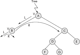
Fig. 7.18 Partial travel of V-L-R order
The travel starts from root node A and its data is processed (V). As it has a left child, we move to B (L) and its data is processed (V). As B has no left child, the right child of B needs to be travelled which is also NULL. Thus, the travel of B is complete and the processing of node A and travel of left sub-tree of A is also over. As per the strategy, the travel moves to its right sub-tree, i.e., to node C (R). The process is repeated for this sub-tree with root node as C. The final trace of the travel is given below:
A B C D F G E
An algorithm for preorder travel (V-L-R) is given below. It is provided with a pointer called Tree that points to the root of the binary tree.
   Algorithm preorderTravel(Tree)
   {
     if (Tree == NULL) return
     else
     { process DATA (Tree);
     preorderTravel (leftChild (Tree));
     preorderTravel (rightChild (Tree));
     }
   }
Example 2: Write a program that creates a generalized binary tree and travels it using preorder strategy. While travelling, it should print the data of the visited node.
Solution: We would use the algorithms createBinTree() and preorderTravel(Tree) to write the program. However, the code will be similar to Example 1. Therefore, only the function preOrderTravel() is provided.
The required program is given below:
   void preOrderTravel (struct tnode *binTree)
   {
    if (binTree == NULL) return;
    printf (“%c ”, binTree->ch);
    preOrderTravel (binTree->leftChild);
    preOrderTravel (binTree->rightChild);
   }
The function has been tested for the binary tree given in Figure 7.15 represented using the following tree list:
treeList[] = {’A’, ’(’, ’B’, ’(’, ’D’,’(’,’H’, ’I’,’)’, ’E’,’(’, ’J’,’$’,’)’,’)’,’C’,’(’,’F’,’(’,’K’,’L’,’)’,’G’,’)’,’)’,’#’};
The output of the program is given below:
A B D H I E J C F K L G
The above output has been tested to be true.
The program was also tested on the following binary tree:
char treeList[] = { ’1’, ’(’,’2’, ’(’, ’$’, ’4’, ’)’,’3’, ’(’,’5’,’6’,’)’,’)’,’#’}
The output of the program is given below:
1 2 4 3 5 6
It is left as an exercise for the students to generate the binary tree from the treeList and then verify the output.
7.4.3.3 Postorder Travel (L-R-V)
This order of travel, i.e., L-R-V requires that while travelling the binary tree, the data of the visited node be processed only after both the left and right sub-trees of a node have been travelled.
Consider the binary tree given in Figure 7.19. Its root node is pointed by a pointer called Tree.
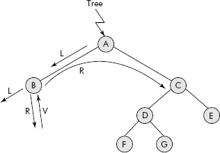
Fig. 7.19 Partial travel of L-R-V order
The travel starts from root node A and its data is not processed as it has a left child which needs to be travelled first indicated by the operation L. Therefore, we move to B. As B has no left child, the right child of B needs to be travelled which is NULL indicated by the operation R. Now, data of node B is processed indicated by the operation V. Thus, the travel of B is complete and the travel of left sub-tree of A is also over. As per the strategy, the travel moves to its right sub-tree, i.e., to node C (R). The process is repeated for this sub-tree with root node as C. The final trace of the travel is given below:
B F G D E C A
An algorithm for postorder travel (L-R-V) is given below. It is provided with the pointer called Tree that points to the root of the binary tree.
   Algorithm postOrderTravel(Tree)
   {
     if (Tree == NULL) return
     else
     { postOrderTravel (leftChild (Tree));
     postOrderTravel (rightChild (Tree));
     process DATA (Tree);
     }
   }
Example 3: Write a program that creates a generalized binary tree and travels it using preorder strategy. While travelling, it should print the data of the visited node.
Solution: We would use the algorithms createBinTree() and postOrderTravel(Tree) to write the program. However, the code will be similar to Example 1. Therefore, only the function postOrderTravel() is provided.
The required function is given below:
   void postOrderTravel (struct tnode *binTree)
   {
     if (binTree == NULL) return;
     postOrderTravel (binTree->leftChild);
     postOrderTravel (binTree->rightChild);
     printf (“%c ”, binTree->ch);
   }
The function has been tested for the binary tree given in Figure 7.15 represented using the following tree list:
treeList[] = {’A’, ’(’, ’B’, ’(’, ’D’,’(’,’H’, ’I’,’)’, ’E’,’(’, ’J’,’$’,’)’,’)’,’C’,’(’,’F’,’(’,’K’,’L’,’)’,’G’,’)’,’)’,’#’};
The output of the program is given below:
H I D J E B K L F G C A
The above output has been tested to be true.
The program was also tested on the following binary tree:
char treeList[] = {’1’, ’(’,’2’, ’(’, ’$’, ’4’, ’)’,’3’, ’(’,’5’,’6’,’)’,’)’,’#’}
The output of the program is given below:
4 2 5 6 3 1
It is left as an exercise for the students to generate the binary tree from the treeList and then verify the output.
7.5 TYPES OF BINARY TREES
There are many types of binary trees. Some of the popular binary trees are discussed in subsequent sections.
7.5.1 Expression Tree
An expression tree is basically a binary tree. It is used to express an arithmetic expression. The reason is simple because both binary tree and arithmetic expression are binary in nature. In binary tree, each node has two children, i.e., left and right child nodes whereas in an arithmetic expression, each arithmetic operator has two operands. In a binary tree, a single node is also considered as a binary tree. Similarly, a variable or constant is also the smallest expression.
Consider the preorder arithmetic expression given below:
* + A * B C − D E
The above arithmetic expression can be expressed as an expression tree given in Figure 7.20.
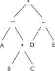
Fig. 7.20 An expression tree of (* + A * B C − D E)
The utility of an expression tree is that the various tree travel algorithms can be used to convert one form of arithmetic expression to another i.e. prefix to infix or infix to post fix or vice-versa.
For example, the inorder travel of the tree given in Figure 7.20 shall produce the following infix expression.
A + B * C * D − E
The postorder travel of the tree given in Figure 7.20 shall produce the following postfix expression:
A B C * + D E − *
Similarly, the preorder travel of the tree given in Figure 7.20 shall produce the following prefix expression:
* + A * B C − D E
From the above discussion, we can appreciate the rationale behind the naming of the travel strategies VLR, LVR, and LRV as preorder, inoder, and postorder, respectively.
Example 4: Write a program that travels the expression tree of Figure 7.21 in an order chosen by the user from a menu. The data of visited nodes are printed. Design an appropriate menu for this program.
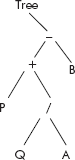
Fig. 7.21 An expression tree
Solution: The expression tree is being expressed as a treeList given below:
treeList = − (+ (P, / (Q, A)), B) #
The above list would be used to write the required menu driven program. The various binary tree travel functions, developed above, would be used to travel the expression tree as per the user choice entered on the following menu displayed to the user:
| Menu | |
| Inorder | 1 |
| Preorder | 2 |
| Postorder | 3 |
| Quit | 4 |
Enter your choice:
The required program is given below:
  /* This program travels an expression tree */
  #include <stdio.h>
  #include <alloc.h>
  #include <conio.h>

  struct tnode
  {
   char ch;
   struct tnode *leftChild, *rightChild;
  };

  struct node
  {
   struct tnode *item;
   struct node * next;
  };

  struct node *push (struct node *Top, struct node *ptr);
  struct node *pop (struct node *Top, struct node **ptr);
  void dispStack(struct node *Top);
  void preOrderTravel (struct tnode *binTree);
  void inOrderTravel (struct tnode *binTree);
  void postOrderTravel (struct tnode *binTree);
  void main ()
  { int i, choice;
    char treeList[] = {’-’, ’(’, ’+’, ’(’, ’P’, ’/’, ’(’, ’Q’, ’A’,’)’,’)’,’B’,’)’,’#’};
    struct node * Top, *ptr, *LChild, *RChild, *Parent;
    struct tnode *binTree;
    int size, tsize;
    size = sizeof (struct node);
    Top =NULL;
    i=0;
    while (treeList[i] != ’#’)
    {
    switch (treeList[i])
    {
    case ’)’:Top = pop (Top, &RChild);
     Top = pop (Top, &LChild);
     Top = pop (Top, &Parent);
     Parent->item->leftChild = LChild->item;
     Parent->item->rightChild =RChild->item;
     Top = push (Top, Parent);
     break;
    case ’(’ :break;
    default:
     ptr = (struct node *) malloc (size);
     if (treeList[i] == ’$’)
     ptr->item = NULL;
     else
     {
      ptr->item->ch = treeList[i];
      ptr->item->leftChild =NULL;
      ptr->item->rightChild =NULL;
      ptr->next = NULL;
     }
     Top = push (Top, ptr);
     break;
    }
    i++;
   }
   Top = pop (Top, &ptr);
                  /* display Menu */
   do {
    clrscr();
    printf (“
 Menu Tree Travel”);
    printf (“

 Inorder 1”);
    printf (“
 Preorder 2”);
    printf (“
 Postorder 3”);
    printf (“
 Quit 4”);
    printf (“

 Enter your choice:”);
    scanf (“%d”, &choice);
    binTree = ptr->item;
    switch (choice)
    {
    case 1: printf(“
 The Tree is..”);
            inOrderTravel(binTree);
            break;
    case 2: printf(“
 The Tree is..”);
            preOrderTravel(binTree);
            break;
    case 3: printf(“
 The Tree is..”);
            postOrderTravel(binTree);
            break;
    };
    printf(“
 Enter any key to continue”);
    getch();
  }
  while (choice != 4);
  }

  struct node * push (struct node *Top, struct node *ptr)
  {
  ptr->next = Top;
  Top = ptr;
  return Top;
  }

  struct node * pop (struct node *Top, struct node **ptr)
  {
    if (Top == NULL) return NULL;
    *ptr = Top;
    Top = Top->next;
    return Top;
  }

  void dispStack(struct node *Top)
  {
   if (Top == NULL)
      printf (“
 Stack Empty”);
   else
   {
    printf (“
 The Stack is: ”);
    while (Top != NULL)
    {
     printf (“ %c ”, Top->item->ch);
     Top =Top->next;
    }
  }
 }

 void preOrderTravel (struct tnode *binTree)
 {
    if (binTree == NULL) return;
    printf (“%c ”, binTree->ch);
    preOrderTravel (binTree->leftChild);
    preOrderTravel (binTree->rightChild);
  }
  void inOrderTravel (struct tnode *binTree)
  {
   if (binTree == NULL) return;
   inOrderTravel (binTree->leftChild);
   printf (“%c ”, binTree->ch);
   inOrderTravel (binTree->rightChild);
  }

  void postOrderTravel (struct tnode *binTree)
  {
   if (binTree == NULL) return;
   postOrderTravel (binTree->leftChild);
   postOrderTravel (binTree->rightChild);
   printf (“%c ”, binTree->ch);
  }
The output of the program for choice 1 (inorder travel) is given below:
The Tree is …: P + Q / A − B
The output of the program for choice 2 (preorder travel) is given below:
The Tree is …: − + P / Q A − B
The output of the program for choice 3 (postorder travel) is given below:
The Tree is …: P Q A / + B −
It is left as an exercise for the readers to verify the results by manually converting the expression to the required form.
7.5.2 Binary Search Tree
As the name suggests, a binary search tree (BST) is a special binary tree that is used for efficient searching of data. In fact a BST stores data in such a way that binary search algorithm can be applied.
The BST is organized as per the following extra conditions on a binary tree:
- The data to be stored must have unique key values.
- The key values of the nodes of left sub-tree are always less than the key value of the root node.
- The key values of the nodes of right sub-tree are always more than the key value of the root node.
- The left and right sub-trees are themselves BSTs.
In simple words we can say that the key contained in the left child is less than the key of its parent node and the key contained in the right child is more than the key of its parent node as shown in Figure 7.22.
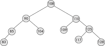
Fig. 7.22 A binary search tree (BST)
Kindly note that the inorder travel of the binary search tree would produce the following node sequence:
Tree is … 83 85 90 104 108 109 110 117 125 128
The above list is sorted in ascending order indicating that a binary search tree is another way to represent and produce a sorted list. Therefore, a binary search algorithm can be easily applied to a BST and, hence, the name, i.e., binary search tree.
7.5.2.1 Creation of a Binary Search Tree
A binary search tree is created by successively reading values for the nodes. The first node becomes the root node. The next node’s value is compared with the value of the root node. If it is less, the node is attached to root’s left sub-tree otherwise to right sub-tree, and so on. When the sub-tree is NULL, then the node is attached there itself. An algorithm for creation of binary search tree is given below.
Note: This algorithm gets a pointer called binTree. The creation of BST stops when an invalid data is inputted. It uses algorithm attach() to attach a node at an appropriate place in BST.
    binTree = NULL; /* initially the tree is empty */

    Algorithm createBST(binTree)
    {
     while (1)
     {
      take a node in ptr
      read DATA (ptr);
      if (DATA (ptr) is not valid) break;
      leftChild (ptr) = NULL;
      rightChild (ptr) = NULL;
      attach (binTree, ptr);
    }
  }
  return binTree;
  }
  Algorithm attach (Tree, node)
  {
   if (Tree == NULL)
   Tree = node;
   else
   {
    if (DATA (node) < DATA(Tree)
    attach (Tree->leftChild);
    else
    attach (Tree-> rightChild);
   }
   return Tree ;
   }
Example 5: Write a program that creates a BST wherein each node of the tree contains non-negative integer. The process of creation stops as soon as a negative integer is inputted by the user. Travel the tree using inorder travel to verify the created BST.
Solution: The algorithm createBST() and its associated algorithm attach() would be used to write the program. The required program is given below:
    /* This program creates a BST and verifies it by travelling it using
    inorder travel */

    #include <stdio.h>
    #include <alloc.h>
    #include <conio.h>

    struct binNode
    {
     int val;
     struct binNode *leftChild, *rightChild;
    };

    struct binNode *createBinTree();
    struct binNode *attach(struct binNode *tree, struct binNode *node);
    void inOrderTravel (struct binNode *binTree);
    void main()
    {
     struct binNode *binTree;
     binTree = createBinTree();
     printf (“
 The tree is...”);
     inOrderTravel(binTree);
    }

    struct binNode *createBinTree()
    {int val, size;
    struct binNode *treePtr, *newNode;
    treePtr = NULL;
    printf (“
 Enter the values of the nodes terminated by a negative value”);
    val = 0;
    size = sizeof (struct binNode);
    while (val >=0)
    {
     printf (“
 Enter val”);
     scanf (“%d”, &val);
     if (val >=0)
     {
      newNode = (struct binNode *) malloc (size);
      newNode->val =val;
      newNode->leftChild =NULL;
      newNode->rightChild=NULL;
      treePtr = attach (treePtr, newNode);
     }
    }
    return treePtr;
    }
   struct binNode *attach(struct binNode *tree, struct binNode *node)
   {
    if (tree == NULL )
    tree = node;
    else
    {
     if (node->val < tree-> val)
      tree->leftChild = attach (tree->leftChild, node);
     else
      tree->rightChild= attach (tree->rightChild, node);
    }
    return tree;
    }

    void inOrderTravel (struct binNode *binTree)
    {
     if (binTree == NULL) return;
     inOrderTravel (binTree->leftChild);
     printf (“%d-”, binTree->val);
     inOrderTravel (binTree->rightChild);
    }
The above program was given the following input:
56 76 43 11 90 65 22
And the following output was obtained when this BST was travelled using inorder travel:
11 22 43 56 65 76 90
It may be noted that the output is a sorted list verifying that the created BST is correct. Similarly, the program was given the following input:
45 12 34 67 78 56
and the following output was obtained:
12 34 45 56 67 78
The output is a sorted list and it verifies that the created BST is correct.
Note: The drawback of a binary search tree is that if the data supplied to the creation process are in a sequence or order then the BST would be a skewed tree. The reason being that every succeeding number being greater than its preceding number would become a right child and would result in a skewed right binary tree. For example, the following input would produce a skewed tree shown in Figure 7.23.
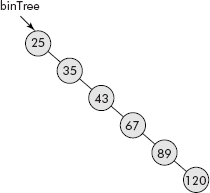
Fig. 7.23 The skewed binary search tree
25 35 43 67 89 120
7.5.2.2 Searching in a Binary Search Tree
The most desirable and important application of a BST is that it is used for searching an entry in a set of values. This method is faster as compared to arrays and linked lists. In an array, the list of items needs to be sorted before a binary search algorithm could be applied for searching an item into the list. On the contrary, the data automatically becomes sorted during the creation of a BST. The item to be searched is compared with the root. If it matches with the data of the root, then success is returned otherwise left or right sub-tree is searched depending upon the item being less or more than the root.
An algorithm for searching a BST is given below; it searches Val in a BST pointed by a pointer called ‘Tree’.
    Algorithm searchBST(Tree, Val)
    {
     if (Tree = NULL)
        return failure;
     if (DATA (Tree) == val)
        return success;
     else
     if (Val < DATA (Tree)
        search (Tree->leftChild, Val);
     else
        search (Tree->rightChild, Val);
    }
Example 6: Write a program that searches a given key in a binary search tree through a function called searchBST(). The function returns 1 or 0 depending upon the search being successful or a failure. The program prompts appropriate messages like “Search successful” or “Search unsuccessful”.
Solution: The above algorithm searchBST() is used. The required program is given below:
   #include <stdio.h>
   #include <alloc.h>
   #include <conio.h>

   struct binNode
   {
    int val;
    struct binNode *leftChild, *rightChild;
   };

   struct binNode *createBinTree();
   struct binNode *attach(struct binNode *tree, struct binNode *node);
   int searchBST (struct binNode *binTree, int val);

   void main()
   { int result, val;
   struct binNode *binTree;
   binTree = createBinTree ();
   printf (“
 Enter the value to be searched”);
   scanf (“%d”, &val);
   result = searchBST(binTree, val);
   if (result == 1)
   printf (“
 Search Successful”);
   else
   printf (“
 Search Un-Successful”);
   }

   struct binNode *createBinTree()
   {
   } /* this function createBinTree() is same as developed in above examples */
   int searchBST (struct binNode *binTree, int val)
   { int flag;
   if (binTree == NULL)
   return 0;
   if (val == binTree->val)
   return 1;
   else
   if (val < binTree-> val)
   flag=searchBST(binTree->leftChild, val);
   else
   flag=searchBST(binTree->rightChild, val);
   return flag;
   }
The above program has been tested.
7.5.2.3 Insertion into a Binary Search Tree
The insertion in a BST is basically a search operation. The item to be inserted is searched within the BST. If it is found, then the insertion operation fails otherwise when a NULL pointer is encountered the item is attached there itself. Consider the BST given in Figure 7.24.
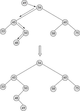
Fig. 7.24 Insertion operation in BST
It may be noted that the number 49 is inserted into the BST shown in Figure 7.24. It is searched in the BST which comes to a dead end at the node containing 48. Since the right child of 48 is NULL, the number 49 is attached there itself.
Note: In fact, a system programmer maintains a symbol table as a BST and the symbols are inserted into the BST in search-insert fashion. The main advantage of this approach is that duplicate entries into the table are automatically caught. The search engine also stores the information about downloaded web pages in search-insert fashion so that possible duplicate documents from mirrored sites could be caught.
An algorithm for insertion of an item into a BST is given below:
    Algorithm insertBST (binTree, item)
    {
     if (binTree == NULL)
     {
       Take node in ptr;
       DATA (ptr) = itm;
       leftChild(ptr) = NULL;
       rightChild(ptr)= NULL;
        binTree = ptr;
        return success;
      }
      else
        if (DATA (binTree) == item)
        return failure;
      else
        { Take node in ptr;
        DATA (ptr) = item;
        leftChild (ptr) = NULL;
        rightChild(ptr)= NULL;
        if (DATA (binTree) > item)
          insertBST (binTree->leftChild, ptr);
        else
          insertBST (binTree->rightChild, ptr);
       }
     }
Example 7: Write a program that inserts a given value in a binary search tree through a function called insertBST(). The function returns 1 or 0 depending upon the insertion being success or a failure. The program prompts appropriate message like “Insertion successful” or “Duplicate value”. Verify the inser-tion by travelling the tree in inorder and displaying its contents containing the inserted node.
Solution: The above algorithm insertBST() is used. The required program is given below:
   /* This program inserts a value in a BST */

   #include <stdio.h>
   #include <alloc.h>
   #include <conio.h>

   struct binNode
   {
   int val;
   struct binNode *leftChild, *rightChild;
   };

   struct binNode *createBinTree();
   struct binNode *attach(struct binNode *tree, struct binNode *node);
   struct binNode * insertBST (struct binNode *binTree, int val, int *flag);
   void inOrderTravel (struct binNode *Tree);
   void main()
   { int result, val;
   struct binNode *binTree;
   binTree = createBinTree ();
   printf (“
 enter the value to be inserted”);
   scanf (“%d”, &val);
   binTree = insertBST(binTree, val, &result);
   if (result == 1)
   { printf (“
 Insertion Successful, The Tree is..”);
   inOrderTravel (binTree);
   }
    else
    printf (“
 duplicate value”);
   }

   struct binNode *createBinTree()
   /* this function createBinTree() is same as developed in above examples */
   {
   }

   struct binNode *attach(struct binNode *tree, struct binNode *node)
   {
     if (tree == NULL )
        tree = node;
     else
     {
    if (node->val < tree-> val)
       tree->leftChild = attach (tree->leftChild, node);
    else
      tree->rightChild= attach (tree->rightChild, node);
   }
   return tree;
  }
  struct binNode * insertBST (struct binNode *binTree, int val, int
  *flag)
  { int size;
  struct binNode *ptr;
  size = sizeof(struct binNode);
  if (binTree == NULL)
  { ptr = (struct binNode *) malloc (size);
  ptr->val = val;
  ptr->leftChild = NULL;
  ptr->rightChild =NULL;
  binTree = ptr;
  *flag=1;
  return binTree;
  }
  if (val == binTree->val)
  {
  *flag= 0;
  return binTree;
  }
  else
  if (val < binTree-> val)
  binTree->leftChild=insertBST(binTree->leftChild, val, flag);
  else
  binTree->rightChild=insertBST(binTree->rightChild, val, flag);
  return binTree;
  }

  void inOrderTravel (struct binNode *Tree)
  {
    if (Tree != NULL)
    {
     inOrderTravel (Tree->leftChild);
     printf (“%d - ”, Tree->val);
     inOrderTravel (Tree->rightChild);
   }
  }
The above program was tested for the following input:
Nodes of the BST: 45 12 67 20 11 56
Value to be inserted: 11
The output: “Duplicate value” was obtained indicating that the value is already present in the BST. Similarly, for the following input:
Nodes of BST: 65 78 12 34 89 77 22
Value to be inserted: 44
The output: Insertion successful, the Tree is .. 12 22 34 44 65 77 78 89, indicating that the insertion at proper place in BST has taken place.
7.5.2.4 Deletion of a Node from a Binary Search Tree
Deletion of a node from a BST is not as simple as insertion of a node. The reason is that the node to be deleted can be at any of the following positions in the BST:
- The node is a leaf node.
- The node has only one child.
- The node is an internal node, i.e., having both the children.
Case 1: This case can be very easily handled by setting the pointer to the node from its parent equal to NULL and freeing the node as shown in Figure 7.25.
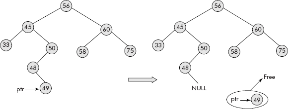
Fig. 7.25 Deletion of a leaf node
The leaf node containing 49 has been deleted. Kindly note that its parent’s pointer has been set to NULL and the node itself has been freed.
Case 2: This case can also be handled very easily by setting the pointer to the node from its parent equal to its child node. The node may be freed later on as shown in Figure 7.26.
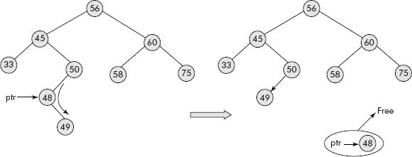
Fig. 7.26 Deletion of a node having only one child
The node, containing 48, having only one child (i.e., 49) has been deleted. Kindly note that its parent’s pointer (i.e., 50) has been set to its child (i.e., 49) and the node itself has been freed.
Case 3: From discussions on BST, it is evident that when a BST is travelled by inorder, the displayed contents of the visited nodes are always in increasing order, i.e., the successor is always greater then the predecessor. Another point to be noted is that inorder successor of an internal node (having both children) will never have a left child and it is always present in the right sub-tree of the internal node.
Consider the BST given in Figure 7.26. The inorder successor of internal node 45 is 48, and that of 56 is 58. Similarly, in Figure 7.22, the inorder successors of internal nodes 90, 108, and 110 are 104, 109, and 117, respectively and each one of the successor node has no left child. It may be further noted that the successor node is always present in the right sub-tree of the internal node.
The successor of a node can be reached by first moving to its right child and then keep going to left till a NULL is found as shown in Figure 7.27.
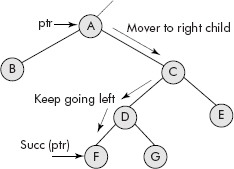
Fig. 7.27 Finding inorder successor of a node
It may be further noted that if an internal node ptr is to be deleted then the contents of inorder successor of ptr should replace the contents of ptr and the successor be deleted by the methods sug-gested for Case 1 or Case 2, discussed above . The mechanism is shown in Figure 7.28.
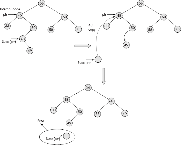
Fig. 7.28 Deletion of an internal node in BST
An algorithm to find the inorder successor of a node is given below. It uses a pointer called succPtr that travels from ptr to its successor and returns it.
    Algorithm findSucc(ptr)
    {
      succPtr = rightChild (ptr);
      while (leftChild (succPtr != NULL)
             succPtr = leftChild (succptr);
      return succPtr;
    }
The algorithm that deletes a node from a BST is given below. It takes care of all the three cases given above.
    Algorithm del NodeBST(Tree, Val)
    {
      ptr = search (Tree, Val); /* Finds the node to be deleted */
      parent = search (Tree, Val); /* Finds the parent of the node */
      if (ptr == NULL) report error and return;

      if (leftChild (ptr) == NULL && rightChild(ptr) == NULL) /* Case 1*/
      {
         if (leftChild (Parent) == ptr)
         leftChild (Parent ) = NULL;
       else
         if (rightChild (Parent) == ptr)
         rightChild (Parent ) = NULL;
         free (ptr);
       }

      if (leftChild (ptr ) != NULL && rightChild(ptr) == NULL) /*Case 2 */
      {
        if (leftChild (Parent) == ptr)
           leftChild (Parent ) = leftChild (ptr);
        else
           if (rightChild (Parent) == ptr)
           rightChild (Parent ) = leftChild (ptr);
        free (ptr);
      }
      else

      if (leftChild (ptr ) == NULL && rightChild(ptr) != NULL) /*Case 2 */
      {
       if (leftChild (Parent) == ptr)
          leftChild (Parent ) = rightChild (ptr);
       else
          if (rightChild (Parent) == ptr)
          rightChild (Parent ) = rightChild (ptr);
       free (ptr);
       }

       if (leftChild (ptr ) != NULL && rightChild(ptr) != NULL) /*Case 3 */
       {
         succPtr = findSucc (ptr);
         DATA (ptr) = DATA (succPtr);
         delNodeBST (Tree, succPtr);
       }
Example 8: Write a program that deletes a given node form binary search tree. The program prompts appropriate message like “Deletion successful”. Verify the deletion for all the three cases by travelling the tree in inorder and displaying its contents.
Solution: The above algorithms del NodeBST() and findSucc() are used. The required program is given below:
   /* This program deletes a node from a BST */

   #include <stdio.h>
   #include <alloc.h>
   #include <conio.h>

   struct binNode
   {
     int val;
     struct binNode *leftChild, *rightChild;
   };

   struct binNode * createBinTree();
   struct binNode *attach(struct binNode *tree, struct binNode *node);
   struct binNode *searchBST (struct binNode *binTree, int val, int    *flag);
   struct binNode *findParent (struct binNode *binTree, struct binNode *ptr);
   struct binNode *delNodeBST (struct binNode *binTree, int val, int    *flag);
   struct binNode *findSucc (struct binNode *ptr);
   void inOrderTravel (struct binNode *Tree);
   void main()
   { int result, val;
   struct binNode *binTree;
   binTree = createBinTree ();
   printf (“
 Enter the value to be deleted”);
   scanf (“%d”, &val);
   binTree = delNodeBST(binTree, val, &result);
   if (result == 1)
   {printf (“
 Deletion successful, The Tree is..”);
   inOrderTravel (binTree);
   }
   else
   printf (“
 Node not present in Tree”);
   }

   struct binNode * createBinTree() /* this function createBinTree() is
   same as developed in above examples */
   {
   }

   struct binNode *attach(struct binNode *tree, struct binNode *node)
   { /* this function attach() is same as developed in above examples    */
   }

   struct binNode * delNodeBST (struct binNode *binTree, int val, int *flag)
   { int size, nval;
   struct binNode *ptr, *parent,*succPtr;
   if (binTree == NULL)
   { *flag =0;
   return binTree;
   }
   ptr = searchBST (binTree, val, flag);
   if (*flag == 1)
   parent = findParent (binTree, ptr);
   else
   return binTree;

   if (ptr->leftChild == NULL && ptr->rightChild == NULL) /* Case 1*/
   {
      if (parent->leftChild == ptr)
         parent->leftChild = NULL;
   else
   if (parent->rightChild == ptr)
       parent->rightChild = NULL;
   free (ptr);
   }

   if (ptr->leftChild != NULL && ptr->rightChild == NULL)
   {
     if (parent->leftChild == ptr)
        parent->leftChild = ptr->leftChild;
     else
        if (parent->rightChild == ptr)
        parent->rightChild = ptr->leftChild;
     free (ptr);
     return binTree;
   }
     else
     if (ptr->leftChild == NULL && ptr->rightChild != NULL)
     {
       if (parent->leftChild == ptr)
       parent->leftChild = ptr->rightChild;
       else
       if (parent->rightChild == ptr)
       parent->rightChild = ptr->rightChild;
       free (ptr);
       return binTree;
     }

     if (ptr->leftChild != NULL && ptr->rightChild != NULL)
     {
       succPtr = findSucc (ptr);
       nval = succPtr->val;
       delNodeBST (binTree, succPtr->val, flag);
       ptr->val = nval;
     }
    return binTree;
    }

    void inOrderTravel (struct binNode *Tree)
    {
     if (Tree != NULL)
     {
      inOrderTravel (Tree->leftChild);
      printf (“%d - ”, Tree->val);
      inOrderTravel (Tree->rightChild);
    }
   }
      struct binNode * findSucc(struct binNode *ptr)
      { struct binNode *succPtr;
        getch();
        succPtr = ptr->rightChild;
        while (succPtr->leftChild != NULL)
        succPtr = succPtr->leftChild ;
        return succPtr;
      }
      struct binNode *searchBST (struct binNode *binTree, int val, int *flag)
      {
        if (binTree == NULL)
        {*flag = 0;
      return binTree;
      }
      else
      {
        if (binTree->val ==val)
        {
         *flag = 1;
         return binTree;
        }
      else
        { if (val < binTree->val)
        return searchBST(binTree->leftChild, val, flag);
      else
        return searchBST(binTree->rightChild, val, flag);
       }
       }
       }
       struct binNode *findParent (struct binNode *binTree, struct        binNode *ptr)
       { struct binNode *pt;
       if (binTree == NULL)
       return binTree;
       else
       {
        if (binTree->leftChild == ptr || binTree->rightChild == ptr )
        { pt = binTree; return pt;}
      else
        { if (ptr->val < binTree-> val)
        pt= findParent(binTree->leftChild, ptr);
      else
        pt= findParent(binTree->rightChild, ptr);
     }
       }
       return pt;
      }
The above program was tested for the following input:
Case 1:
Nodes of the BST: 38 27 40 11 39 30 45 28
Value to be deleted: 11, a leaf node
The output: “Deletion successful"-The Tree is.. 27 28 30 38 39 40 45 was obtained.
Case 2:
Similarly, for the following input:
Nodes of BST: 38 27 40 11 39 30 45 28
Value to be deleted: 30, a node having no right child.
The output: Deletion successful, the Tree is.. 11 27 28 38 39 40 45, indicating that the non-leaf node 30 having only one child has been deleted.
Case 3:
Similarly, for the following input:
Nodes of BST: 38 27 40 11 39 30 45 28
Value to be deleted: 40, an internal node having both the children.
The output: Deletion successful, the Tree is.. 11 27 28 30 38 39 45, indicating that the internal node 40 having no child has been deleted.
7.5.3 Heap Trees
A heap tree is a complete binary tree. This data structure is widely used for building priority queues. Sorting is another application in which heap trees are employed; the sorting method is known as heap sort. As the name suggests, a heap is a collection of partially ordered objects represented as a binary tree. The data at each node in heap tree is less than or equal to the data contained in its left child and the right child as shown in Figure 7.29. This property of each node having data part less than or equal to its children is called heap-order property.
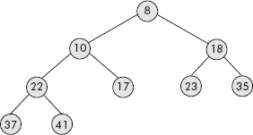
Fig. 7.29 A min-heap tree
As we go from leaf nodes to the root (see Figure 7.29), data of nodes starts decreasing and, therefore, the root contains the minimum data value of the tree. This type of heap tree is called a ’min heap’.
On the contrary, if a node contains data greater than or equal to the data contained in its left and right child, then the heap is called as ‘max heap’. The reason being that as we move from leaf nodes to the root, the data values increase and, therefore, in a max heap the data in the root is the maximum data value in the tree as shown in Figure 7.30.
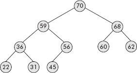
Fig. 7.30 A max-heap tree
A complete binary tree is called a heap tree (say max heap) if it has the following properties:
- Each node in the heap has data value more than or equal to its left and right child nodes.
- The left and right child nodes themselves are heaps.
Thus, every successor of a node has data value less than or equal to the data value of the node. The height of a heap with N nodes = |log 2 N|.
7.5.3.1 Representation of a Heap Tree
Since a heap tree is a complete binary tree, it can be comfortably and efficiently stored in an array. For example, the heap of Figure 7.30 can be represented in an array called ‘heap’ as shown in Figure 7.31. The zeroth position contains total number of elements present in the heap. For example, the zeroth location of heap contains 10 indicating that there are 10 elements in the heap shown in Figure 7.31.
Fig. 7.31 Linear representation of a heap tree
It may be noted that this representation is simpler than the linked representation as there are no links. Moreover from any node of the tree, we can move to its parent or to its children, i.e., in both forward and backward directions. As discussed in Section 7.4.1, the following relationships hold good:
In an array of size N, for the given node i, the following relationships are valid in linear representation:
- leftChild (i) = 2*i {When 2*i > N then there is no left child}
- rightChild(i) = 2*i + 1 {When 2*i +1 > N then there is no right child}
- parent (i) = | i/2 | {node 0 has no parent – it is a root node}
The operations that are defined on a heap tree are:
- Insertion of a node into a heap tree
- Deletion of a node from a heap tree
A discussion on these operations is given in the subsequent sections.
7.5.3.2 Insertion of a Node into a Heap Tree
The insertion operation is an important operation on a heap tree. The node to be inserted is placed on the last available location in the heap, i.e., in the array. Its data is compared with its parent and if it is more than its parent, then the data of both the parent and the child are exchanged. Now the parent becomes a child and it is compared with its own parent and so on; the process stops only when the data part of child is found less than its parent or we reach to the root of the heap. Let us try to insert ‘69’ in the heap given in Figure 7.31. The operation is illustrated in Figure 7.32.
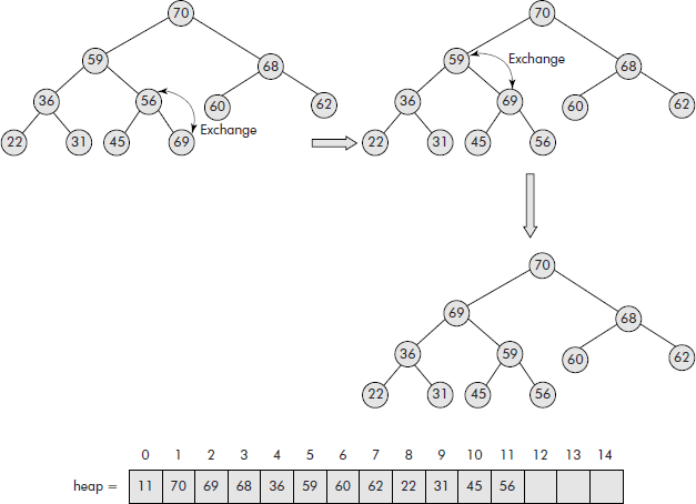
Fig. 7.32 Insertion of a node into a heap tree
An algorithm that inserts an element called item into a heap represented in an array of size N called maxHeap is given below. The number of elements currently present in the heap is stored in the zeroth location of maxHeap.
   Algorithm insertHeap(item)
   {
     if (heap [0] == 0)
     { heap[0] = 1;
     heap[1] = item;
     }
     else
     {
       last = heap[0] +1;
       if (last >size)
          prompt message "Heap Full”;
       else
       {
        heap[last] = item;
        heap[0] = heap [0] +1;
        I = last;
        Flag = 1;
        while (Flag)
        {
         J = abs (I/2); /* find parent’s index */
         if (J >= 1)
         {
          if (heap[J] < heap [I])
          {
           temp = heap[J];
           heap [J]= heap [I];
           heap [I] = temp; /* Parent becomes child */
           I =J;
          }
          else
          Flag = 0;
          }
          else
          Flag=0;
       }
      }
     }
    }
  }
Note: The insertion operation is important because the heap itself is created by iteratively inserting the various elements starting from an empty heap.
Example 9: Write a program that constructs a heap by iteratively inserting elements input by a user into an empty heap.
Solution: The algorithm insertHeap() would be used. The required program is given below:
   /* This program creates a heap by iteratively inserting elements into a heap Tree */

   #include <stdio.h>
   #include <conio.h>
   void insertHeap(int heap[], int item, int size);
   void dispHeap (int heap[]);
   void main()
   {
    int item, i, size;
    int maxHeap [20];
    printf (“
 Enter the size(<20) of heap”);
    scanf (“%d”, &size);
    printf (“
 Enter the elements of heap one by one”);
    for (i=1; i<=size; i++)
   {
    printf (“
 Element:”);
    scanf (“%d”, &item);
    insertHeap(maxHeap, item, size);
   }
    printf (“
 The heap is..”);
    dispHeap(maxHeap);
   }

   void insertHeap(int heap[],int item, int size)
   { int last, I, J, temp, Flag;
   if (heap [0] == 0)
   { heap[0] = 1;
   heap[1] = item;
   }
   else
   {
    last = heap[0] + 1;
    if (last >size)
    {
     printf (“
 Heap Full”);
    }
    else
    {
     heap[last] = item;
     heap[0]++;
     I = last;
     Flag = 1;
     while (Flag)
     {
       J = (int) (I/2);
       if (J >= 1)
       { /* find parent */
         if (heap[J] < heap [I])
         {
          temp = heap[J];
          heap [J]= heap [I];
          heap [I] = temp;
          I =J;
         }
         else
          Flag = 0;
       }
        else
         Flag=0;
      }
   }
  }
  }

  void dispHeap (int heap[])
  {
   int i;
   for (i = 1; i <= heap[0]; i++)
       printf (“%d ”, heap[i]);
  }
The above program was tested for the input: 22 15 56 11 7 90 44
The output obtained is: 90 15 56 11 7 22 44, which is found to be correct.
In the next run, 89 was added to the list, i.e., 22 15 56 11 7 90 44 89.
We find that the item ‘89’ has been inserted at proper place as indicated by the output obtained thereof: 90 89 56 15 7 22 44 11
It is left as an exercise for the reader to verify above results.
7.5.3.3 Deletion of a Node from a Heap Tree
The deletion operation on heap tree is relevant when its root is deleted. Deletion of any other element has insignificant applications. The root is deleted by the following steps:
Step
- Save the root in temp.
- Bring the right most leaf of the heap into root.
- Move root down the heap till the heap is ordered.
- Return temp containg the deleted node.
The operation, given in step2 above is also called reheap operation. Consider the heap given in Figure 7.33.
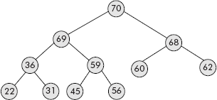
Fig. 7.33 A heap tree
Let us delete its root (i.e., 70) by bringing the rightmost leaf (i.e., 56) into the root as shown in Figure 7.34. The root has been saved in temp.
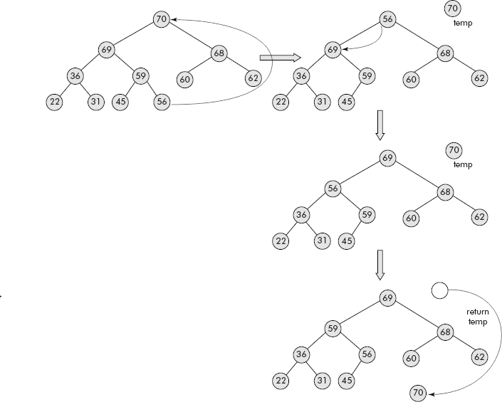
Fig. 7.34 Deletion of root from a heap
An algorithm that deletes the maximum element (i.e., root) from a heap represented in an array of size N called maxHeap is given below. The number of elements currently present in the heap is stored in the zeroth location of maxHeap.
   Algorithm delMaxHeap(heap)
   {
     if (heap[0] == 1) return heap[1]; /* There is only one element in the heap */
     last = heap[0];
     tempVal = heap[1]; /* Save the item to be deleted and returned */
     heap[1]= heap[last]; /* Bring the last leaf node to root */
     heap[0]--; /* Reduce the number of elements by 1 */
     K = last − 1;
     I=1; /* Point to root */
     Flag = 1;
     while (Flag)
     {
      J = I*2;
      if (J <= K)
      { /* find bigger child and store its position in pos */
       if (heap[J] > heap[J+1])
       pos = J;
       else
        pos = J+1;
       if (heap [pos] > heap[I]) /* perform reheap */
       {
        temp = heap[pos];
        heap [pos]= heap [I];
        heap [I] = temp;
        I =pos; /* parent becomes the child */
       }
       else
        Flag = 0;
       }
       else
        Flag=0;
     }
     return tempVal;
   }
Example 10: Write a program that deletes and displays the root of a heap. The remaining elements of the heap are put to reheap operation.
Solution: The algorithm delMaxHeap() would be used. The required program is given below:
   /* This program deletes the maximum element from a heap Tree*/

   #include <stdio.h>
   #include <conio.h>
   int delMaxHeap(int heap[]);
   void insertHeap(int heap[],int item, int size);
   void dispHeap(int heap[]);
   void main()
   {
    int item, i, size;
    int maxHeap [20];
    printf (“
 Enter the size(<20) of heap”);
    scanf (“%d”, &size);
    printf (“
 Enter the elements of heap one by one”);
    for (i=1; i<=size; i++)
    {
      printf (“
 Element :”);
      scanf (“%d”, &item);
      insertHeap(maxHeap, item, size);
    }
    printf (“
 The heap is..”);
    dispHeap(maxHeap);
    item = delMaxHeap(maxHeap);
    printf (“
 The deleted item is : %d”, item);
    printf (“
 The heap after deletion is..”);
    dispHeap(maxHeap);
   }

   void insertHeap(int heap[],int item, int size)
   { int last, I, J, temp, Flag;
   if (heap [0] == 0)
   { heap[0] = 1;
   heap[1] = item;
   }
   else
   {
    last = heap[0] +1;
    if (last >size)
    {
     printf (“
 Heap Full”);
    }
    else
    {
     heap[last] = item;
     heap[0]++;
     I = last;
     Flag = 1;
     while (Flag)
     {
      J = (int) (I/2);
      if (J >= 1)
      { /* find parent */
         if (heap[J] < heap [I])
         {
         temp = heap[J];
         heap [J]= heap [I];
         heap [I] = temp;
         I =J;
      }
      else
         Flag = 0;
      }
      else
         Flag=0;
     }
    }
   }
   }
   void dispHeap (int heap[])
   {
    int i;
    for (i = 1; i <= heap[0]; i++)
    printf (“%d ”, heap[i]);
  }
  int delMaxHeap(int heap[])
    {
     int temp, I, J, K, val, last, Flag, pos;
     if (heap[0] == 1) return heap[1];
     last = heap[0];
     val = heap[1];
     heap[1]= heap[last];
     heap[0]--;
     K = last − 1;
     I=1;
     Flag = 1;
     while (Flag)
     {
      J = I*2;
      if (J <= K)
      { /* find child */
        if (heap[J] > heap[J+1])
        pos = J;
      else
       pos = J+1;
      if (heap [pos] > heap[I])
      {
          temp = heap[pos];
          heap [pos]= heap [I];
          heap [I] = temp;
        I =pos;
      }
      else
         Flag = 0;
      }
      else
          Flag=0;
     }
     return val;
   }
The above program was tested for input: 34 11 56 78 23 89 12 5 and the following output was obtained:
The heap is: 89 56 78 11 23 34 12 5
The deleted item is: 89
The heap after deletion is : 78 56 34 11 23 5 12
It is left as an exercise for the students to verify the results by manually making the heaps before and after deletion of the root.
7.5.3.4 Heap Sort
From discussion on heap trees, it is evident that the root of a maxHeap contains the largest value. When the root of the max heap is deleted, we get the largest element of the heap. The remaining elements are put to reheap operation and we get a new heap. If the two operations delete and reheap operation is repeated till the heap becomes empty and the deleted elements stored in the order of their removal, then we get a sorted list of elements in descending order as shown in Figure 7.35.
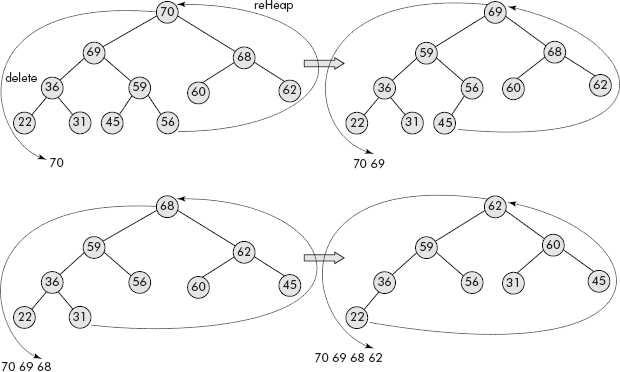
Fig. 7.35 Repetitive deletion from a heap produces sorted list
Example 11: Write a program that sorts a given list of numbers by heap sort.
Solution: We would modify the program of Example 10 wherein the element deleted from heap would be stored in a separate array called sortList. The deletion would be carried out iteratively till the heap becomes empty. Finally, sortList would be displayed. The required program is given below:
    /* This program sorts a given list of numbers using a heap tree*/

    #include <stdio.h>
    #include <conio.h>
    int delMaxHeap(int heap[]);
    void insertHeap(int heap[],int item, int size);
    void dispHeap (int heap[]);
    void main()
    {
     int item, i, size, last;
     int maxHeap [20];
     int sortList [20];
     printf (“
 Enter the size(<20) of heap”);
     scanf (“%d”, &size);
     printf (“
 Enter the elements of heap one by one”);
     for (i=1; i<=size; i++)
     {
      printf (“
 Element :”);
      scanf (“%d”, &item);
      insertHeap(maxHeap, item, size);
     }
     printf (“
 The heap is..”);
     dispHeap(maxHeap);
     getch();
     last = maxHeap[0];
     for (i =0; i < last; i++)
     {
       item = delMaxHeap(maxHeap);
       sortList [i] =item;
     }
     printf (“
 The sorted list...”);
     for (i = 0; i < last; i++)
       printf (“%d ”, sortList[i]);
    }

    void insertHeap(int heap[],int item, int size)
    { int last, I, J, temp, Flag;
    if (heap [0] == 0)
    { heap[0] = 1;
    heap[1] = item;
    }
    else
    {
      last = heap[0] +1;
      if (last >size)
      {
       printf (“
 Heap Full”);
      }
      else
      {
        heap[last] = item;
        heap[0]++;
        I = last;
        Flag = 1;
       while (Flag)
       {
        J = (int) (I/2);
        if (J >= 1)
        { /* find parent */
          if (heap[J] < heap [I])
          {
           temp = heap[J];
           heap [J]= heap [I];
           heap [I] = temp;
           I =J;
           }
           else
             Flag = 0;
          }
          else
            Flag=0;
        }
       }
     }
     }

     void dispHeap (int heap[])
     {
      int i;
      for (i = 1; i <= heap[0]; i++)
           printf (“%d ”, heap[i]);
     }
     int delMaxHeap(int heap[])
     {
       int temp, I, J, K, val, last, Flag, pos;
       if (heap[0] == 1) return heap[1];
       last = heap[0];
       val = heap[1];
       heap[1]= heap[last];
       heap[0]−−;
       K = last − 1;
       I=1;
       Flag = 1;
       while (Flag)
       {
        J = I*2;
        if (J <= K)
        { /* find child */
         if (heap[J] > heap[J+1])
            pos = J;
       else
         pos = J+1;
       if (heap [pos] > heap[I])
       {
        temp = heap[pos];
        heap [pos]= heap [I];
        heap [I] = temp;
        I = pos;
       }
       else
        Flag = 0;
     }
     else
        Flag=0;
    }
    return val;
   }
The above program was tested for the input: 87 45 32 11 34 78 10 31
The output obtained is given below:
The heap is: 87 45 78 31 34 32 10 11
The sorted list is … 87 78 45 34 32 31 11 10
Thus, the program has performed the required sorting operation using heap sort.
Note: The above program is effective and gives correct output but it is inefficient from the storage point of view. The reason being that it is using an extra array called sortList to store the sorted list.
The above drawback can be removed by designing an in-place heap sort algorithm that uses the same array to store the sorted list in which the heap also resides. In fact, the simple modification could be that let root and the last leaf node be exchanged. Without disturbing the last node, reheap the remaining heap. Repeat the exchange and reheap operation iteratively till only one element is left in the heap. Now, the heap contains the elements in ascending order. The mechanism is illustrated in Figure 7.36.
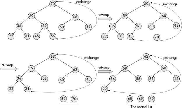
Fig. 7.36 The in-place heap sort
    Algorithm IpHeapSort()
    {
       if (heap[0] > 1)
       {
       do
       {
         last = heap[0];
         temp = heap[1]; /* exchange root and last leaf node*/
         heap[1] = heap[last];
         heap[last] = temp;
         heap[0]−−;
         last = heap[0]; /* last points to new last leaf node */
         K = last − 1;
         I=1;
         Flag = 1;
         while (Flag)
         {
          J = I*2;
          if (J <= K)
          { /* find child which is greater than parent*/
           if (heap[J] > heap[J+1])
           pos = J;
          else
           pos = J+1;
           if (heap [pos] > heap[I])
         {
           temp = heap[pos]; /* exchange parent and child */
           heap [pos]= heap [I];
           heap [I] = temp;
           I =pos;
         }
          else
            Flag = 0;
         }
           else
           Flag=0;
        }
     }
     while (last >1);
   }
  }
It may be noted that the element at the root is being exchanged with the last leaf node and the rest of the heap is being put to reheap operation. This is iteratively being done in the do-while loop till there is only one element left in the heap.
Example 12: Write a program that in-place sorts a given list of numbers by heap sort.
Solution: We would employ the algorithm IpHeapSort() wherein the element from the root is exchanged with the last leaf node and rest of the heap is put to reheap operation. The exchange and reheap is carried out iteratively till the heap contains only 1 element.
The required program is given below:
   /* This program in place sorts a given list of numbers using heap tree*/

   #include <stdio.h>
   #include <conio.h>
   void sortMaxHeap(int heap[]);
   void insertHeap(int heap[],int item, int size);
   void dispHeap (int heap[]);
   void main()
   {
    int item, i, size, last;
    int maxHeap [20];
    printf (“
 Enter the size(<20) of heap”);
    scanf (“%d”, &size);
    printf (“
 Enter the elements of heap one by one”);
    for (i=1; i<=size; i++)
    {
     printf (“
 Element :”);
     scanf (“%d”, &item);
     insertHeap(maxHeap, item, size);
    }
    printf (“
 The heap is..”);
    dispHeap(maxHeap);
    getch();
    sortMaxHeap(maxHeap);
    printf (“
 The sorted list...”);
    for (i = 1; i <= size; i++)
         printf (“%d ”, maxHeap[i]);
   }

   void insertHeap(int heap[],int item, int size)
   { int last, I, J, temp, Flag;
   if (heap [0] == 0)
   { heap[0] = 1;
   heap[1] = item;
   }
   else
   {
    last = heap[0] +1;
    if (last >size)
    {
     printf (“
 Heap Full”);
    }
   else
   {
    heap[last] = item;
    heap[0]++;
    I = last;
    Flag = 1;
    while (Flag)
    {
     J = (int) (I/2);
     if (J >= 1)
     { /* find parent */
     if (heap[J] < heap [I])
     {
       temp = heap[J];
       heap [J]= heap [I];
       heap [I] = temp;
       I =J;
     }
     else
        Flag = 0;
     }
     else
        Flag=0;
     }
    }
    }
    }

    void dispHeap (int heap[])
    {
     int i;
     for (i = 1; i <= heap[0]; i++)
          printf (“%d ”, heap[i]);
    }
    void sortMaxHeap(int heap[])
    {
     int temp, I, J, K, val, last, Flag, pos;
     if (heap[0] > 1)
     {
      do
      {
       last = heap[0];
       temp = heap[1]; /*Exchange root with the last node */
       heap[1] = heap[last];
       heap[last] = temp;
       heap[0]−−;
       last = heap[0];
       K = last −1;
       I=1;
       Flag = 1;
       while (Flag)
       {
        J = I*2;
        if (J <= K)
        { /* find child */
           if (heap[J] > heap[J+1])
           pos = J;
        else
           pos = J+1;
           if (heap [pos] > heap[I])
        {
           temp = heap[pos];
           heap [pos]= heap [I];
           heap [I] = temp;
           I =pos;
        }
        else
           Flag = 0;
        }
        else
           Flag=0;
      }
    }
    while (last >1);
   }
  }
7.5.3.5 Merging of Two Heaps
Merging of heap trees is an interesting application wherein two heap trees are merged to produce a tree which is also a heap. The merge operation is carried out by the following steps:
Given two heap trees: Heap1 and Heap2
Step
- Delete a node from Heap2.
- Insert the node into Heap1.
- Repeat steps 1 and 2 till Heap 2 is not empty.
Consider the merge operation shown in Figure 7.37.
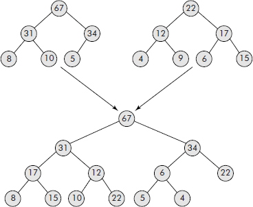
Fig. 7.37 Merging of two heap trees
Example 13: Write a program that merges two heap trees to produce a third tree which is also a heap.
Solution: The required program is given below:
   /* This program merges two heap trees */

   #include <stdio.h>
   #include <conio.h>
   int delMaxHeap(int heap[]);
   void insertHeap(int heap[], int item, int size);
   void dispHeap (int heap[]);
   void main()
   {
    int item,i,size1, size2;
    int maxHeap1 [20],maxHeap2[20];
    printf (“
 Enter the size(<20) of heap1”);
    scanf (“%d”, &size1);
    printf (“
 Enter the elements of heap one by one”);
    for (i=1; i<=size1; i++)
    {
      printf (“
 Element :”);
      scanf (“%d”, &item);
      insertHeap(maxHeap1, item, size1);
    }
    printf (“
 The heap1 is..”);
    dispHeap(maxHeap1);
    printf (“
 Enter the size(<20) of heap2”);
    scanf (“%d”, &size2);
    printf (“
 Enter the elements of heap one by one”);
    for (i=1; i<=size2; i++)
    {
      printf (“
 Element :”);
      scanf (“%d”, &item);
      insertHeap(maxHeap2, item, size2);
    }
    printf (“
 The heap2 is..”);
    dispHeap(maxHeap2);
    for (i = 1; i <= size2; i++)
    {
     item = delMaxHeap(maxHeap2);
     size1=size1+1;
     insertHeap (maxHeap1, item,size1);
    }
    printf (“
 The heaps after merge is..”);
    dispHeap(maxHeap1);
    }

    void insertHeap(int heap[], int item, int size)
    { int last, I, J, temp, Flag;
    if (heap [0] == 0)
    { heap[0] = 1;
    heap[1] = item;
    }
    else
    {
      last = heap[0] +1;
      if (last >size)
    {
    printf (“
 Heap Full”);
    }
    else
    {
     heap[last] = item;
     heap[0]++;
     I = last;
     Flag = 1;
     while (Flag)
     {
      J = (int) (I/2);
      if (J >= 1)
      {  /* find parent */
       if (heap[J] < heap [I])
       {
        temp = heap[J];
        heap [J]= heap [I];
        heap [I] = temp;
        I =J;
       }
       else
       Flag = 0;
       }
       else
       Flag=0;
     }
    }
   }
  }

  void dispHeap (int heap[])
  {
    int i;
    for (i = 1; i <= heap[0]; i++)
        printf (“%d ”, heap[i]);
  }
  int delMaxHeap(int heap[])
  {
    int temp, I, J, K, val, last, Flag, pos;
    if (heap[0] == 1) return heap[1];
    last = heap[0];
    val = heap[1];
    heap[1]= heap[last];
    heap[0]−−;
    K = last −1;
    I=1;
    Flag = 1;
    while (Flag)
    {
     J = I*2;
     if (J <= K)
     { /* find child */
        if (heap[J] > heap[J+1])
        pos = J;
     else
        pos = J+1;
     if (heap [pos] > heap[I])
     {
        temp = heap[pos];
        heap [pos]= heap [I];
        heap [I] = temp;
        I =pos;
     }
     else
        Flag = 0;
     }
     else
         Flag=0;
    }
    return val;
   }
The above program was tested on the heap trees given in Figure 7.37. The input provided is given below:
Heap1: 67 31 34 8 10 5
Heap2: 22 12 17 4 9 615
The output obtained is given below:
The heap after merge is …67 31 34 17 12 6 22 8 15 10 9 5 4
It is left for the reader to verify the output from Figure 7.37.
Note: Both MaxHeap and MinHeap trees can be merged. The type of output merged tree will depend upon the type of Heap1. If Heap1 is maxHeap, then the heap obtained after merge operation would also be of type maxHeap. Similarly, if Heap1 is minHeap, then the heap obtained after merge operation would also be of type minHeap.
7.5.4 Threaded Binary Trees
From the discussion on binary trees, it is evident that creation of a tree is a one time process. But, a tree is travelled numerous times consuming a large part of the overall time taken by an algorithm. Moreover, the travel algorithms are recursive in nature amounting to large usage of storage. Therefore, there is a scope for reducing the travels or the number of steps required to travel a tree. For example, during inor-der travel, we move from a node to its successor and from the successor to its successor, and so on.
The questions is can we move directly to an inorder successor of a node in a tree. The answer is yes if we can keep pointers from the nodes to their successors and move through the tree using these pointers.
We know that in a binary tree of N nodes, there are ‘N + 1’ NULL pointers. Therefore, the unused NULL pointers of the binary tree can be employed for the purpose of non-recursive travelling within a binary tree. Let us modify the structure of the node of binary tree as per the following rules:
- If a node is having an empty left child (i.e., a NULL pointer), then replace it by a special pointer that points to its predecessor node in the tree.
- If a node is having an empty right child (i.e., a NULL pointer), then replace it by a special pointer that points to its successor node in the tree.
- The special pointer is called a thread.
Consider the binary tree given in Figure 7.38 wherein a binary tree has been assigned the threads. It may be noted that the normal pointers have been shown with thick lines and the threads with dotted lines.
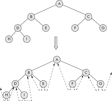
Fig. 7.38 The vacant NULL pointers have been replaced by threads
The resultant binary tree of Figure 7.38 is called a threaded binary tree (TBT). It may be noted that the characteristic of this special tree is that a left thread of a node points to its inorder predecessor and the right thread to its inorder successor. For example, the left thread of ‘E’ is pointing to ‘B’, its predecessor and the right thread of ‘E’ is pointing to ‘A’, its successor.
A threaded binary tree is a binary tree in which a node uses its empty left child pointer to point to its inorder predecessor and the empty right child pointer to its inorder successor.
Now, the problem is that how a program would differentiate between a normal pointer and a thread. A simple solution is to keep variables called LTag and RTag, having value 1 or 0 indicating a normal pointer or a thread, respectively. Accordingly, a node of a threaded binary tree would have the structure as given in Figure 7.39.
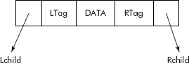
Fig. 7.39 A node of a threaded binary tree
Let us now use the structure of Figure 7.39 to represent the threaded binary tree of Figure 7.38. The arrangement is shown in Figure 7.40.
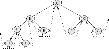
Fig. 7.40 The threaded binary tree with node structure having the Tag bits
A left thread pointing to NULL indicates that there is no more inorder predecessor. Similarly, a NULL right thread indicates that there is no more inorder successor. For example, the left thread of ‘H’ is pointing to NULL and the right thread of ‘G’ is pointing to NULL. This anomalous situation can be handled by keeping a head node having a left child and a right thread as shown in Figure 7.41. This dummy node does not contain any value. In fact, it is an empty threaded binary tree because both its left child and right thread are pointing to itself.
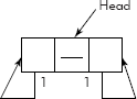
Fig. 7.41 A head node indicating an empty threaded binary tree
Now the dangling threads of a binary tree can be made to point to the head node and the left child of the head node to the root of the binary threaded tree as shown in Figure 7.42.
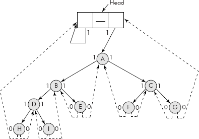
Fig. 7.42 A binary threaded tree with a head node
Now with the arrangement shown in Figure 7.42, it can be appreciated that an inorder successor of a node pointed by ptr can be very easily found by the following set of rules:
- If RTag of ptr is 0, then the rightChild is pointing to its successor.
- If RTag of ptr is 1 (i.e., thread), then the left most node of its right sub-tree is its successor.
An algorithm that returns inorder successor of a node is given below:
   Algorithm findSucc(ptr)
   {
    if (RTag (ptr) == 0)
       return rightChild (ptr);
    else
    {
       ptr = rightChild (ptr)
       while (LTag (ptr) =1)
       ptr = leftChild(ptr);
    }
    return ptr;
   }
Similarly, an inorder predecessor of a node pointed by ptr can be very easily found by the following set of rules:
- If LTag of ptr is 0, then the leftChild is pointing to its predecessor.
- If LTag of ptr is 1 (i.e., thread), then the right most node of its left sub-tree is its predecessor.
An algorithm that returns inorder successor of a node is given below:
   Algorithm findPred(ptr)
   {
     if (LTag (ptr) == 0)
        return leftChild (ptr);
     else
     {
        ptr = leftChild (ptr)
        while (RTag (ptr) =1)
        ptr = rightChild(ptr);
     }
     return ptr;
   }
Now we can write an algorithm for non-recursive inorder travel of a threaded binary tree (TBT), which is given below:
   Algorithm inOrderTBT(Tree)
   {
    Tree = Head;
    while (1)
   {
     tree = findSucc(tree);
     if (tree = Head) return;
     else
     print DATA (Tree);
   }
  }
The following operations can be defined on a threaded binary tree.
- Insertion of a node into a TBT.
- Deletion of a node from a TBT.
As the threaded binary tree has been designed to honour inorder travel, the insertion and deletion have to be carried out in such a way that after the operation the tree remains the inorder threaded binary tree. A brief discussion on both the operations is given in the subsequent sections.
7.5.4.1 Insertion into a Threaded Binary Tree
A node ‘X’, having Data part equal to ‘T’, can be inserted into an inorder threaded binary tree after node ‘Y’ in either of the following four ways:
Case 1: - When X is inserted as left child of Y and Y has an empty left child.
Case 2: - When X is inserted as right child of Y and Y has an empty right child.
Case 3: - When X is inserted as left child of Y and Y has a non-empty left child
Case 4: - When X is inserted as right child of Y and Y has a non-empty right child.
CASE 1:
When Y (Say Data part equal to ‘F’) has an empty left child, then it must be a thread. The insertion can be made by making the left thread of X (Data part equal to ‘T’) to point where the left thread of Y is currently pointing to. Thereafter, X becomes the left child of Y for which LTag of Y is reset to 1. The right child of X is set as thread pointing to the node Y, indicating that Y is the successor of X. The insertion operation is shown in Figure 7.43.
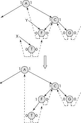
Fig. 7.43 Insertion of a node X after Y having no left child
It may be noted that the node containing ‘T’ has become the left child of node containing ‘F’. After the insertion, the tree is still a threaded binary tree. The predecessor of ‘T’ is ‘A’ and the successor of ‘T’ is ‘F’.
An algorithm for insertion of node as left thread is given below:
   Algorithm insertAtLThread(X,Y)
   {
     if (LTag(Y) == 0)
     {
       LTag (X) =0;
       leftChild (X) = leftChild (Y);
       LTAg (Y) =1;
       leftChild (Y) = X;
       RTag (X) = 0;
       rightChild (X) = Y;
    }
   }
CASE 2:
When Y (Data part equal to ‘F’) has an empty right child, then it must be a thread. The insertion can be made by making the right thread of X (Data part equal to ‘T’) to point where the right thread of Y is currently pointing to. Thereafter, X becomes the right child of Y for which RTag of Y is reset to 1. The left child of X is set as a thread pointing to the node Y, indicating that Y is the predecessor of X. The insertion operation is given in Figure 7.44.
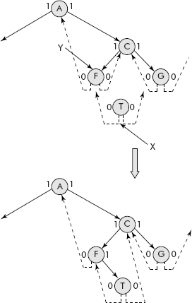
Fig. 7.44 Insertion of a node X after Y having no right child
It may be noted that the node containing ‘T’ has become the right child of node containing ‘F’. After the insertion, the tree is still a threaded binary tree. The predecessor of ‘T’ is ‘F’ and the successor of ‘T’ is ‘C’.
An algorithm for insertion of node as right thread is given below:
   Algorithm inserAtRThread(X,Y)
   {
    if (RTag(Y) == 0)
    {
     RTag (X) =0;
     rightChild (X) = rightChild (Y);
     RTAg (Y) =1;
     rightChild (Y) = X;
     LTag (X) = 0;
     leftChild (X) = Y;
    }
   }
CASE 3:
When Y (Data part equal to ‘C’) has non-empty left child, the insertion can be made by making the left child of X (Data part equal to ‘T’) point where the left child of Y is currently pointing to. Thereafter, X becomes the left child of Y for which Lchild of Y is pointed to X. The right child of X is set as thread pointing to the node Y, indicating that Y is the successor of X.
Now the most important step is to find the inorder predecessor of Y (pointed by ptr) and make it inorder predecessor of X by making ptr’s right thread to point to X. The insertion operation is shown in Figure 7.45.
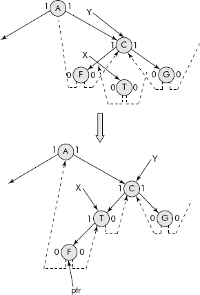
Fig. 7.45 Insertion of a node at non empty left child of a given node
It may be noted that the node containing ‘T’ has become the left child of node containing ‘C’. After the insertion, the tree is still a threaded binary tree. The predecessor of ‘T’ is ‘F’ and the successor of ‘T’ is ‘C’.
An algorithm for insertion of node as left child is given below:
   Algorithm insertAtLchild(X,Y)
   {
    RTag (X) =0;    /* Connect the right thread of X to Y */
    rightChild (X) = Y
    LTAG (X) = 1;   /* Connect the leftChild of X to the node pointed by
    left child o Y */
    leftChild (X) = leftChild (Y)
                    /* Point the left child of Y to X */
    leftChild (Y) = X;
    ptr = inOrderPred (Y)   /* Find the inorder predecessor of Y */
    rightChild (ptr) =X;    /* Connect the right thread of (ptr) predecessor
    to X */
   }
CASE 4:
When Y (Data part equal to ‘C’) has non-empty right child, the insertion can be made by making the right child of X (Data part equal to ‘T’) point where the right child of Y is currently pointing to. There-after, X becomes the right child of Y by pointing the right child of Y to X. The left thread of X is set as a thread pointing to the node Y, indicating that Y is the predecessor of X.
Now, the most important step is to find the inorder successor of Y (pointed by ptr) and make it inorder successor of X by making ptr’s left thread point to X. The insertion operation is shown in Figure 7.46.
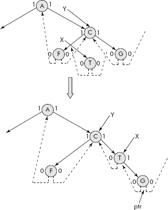
Fig. 7.46 Insertion of a node at non-empty right child of a given node
It may be noted that the node containing ‘T’ has become the right child of node containing ‘C’. After the insertion, the tree is still a threaded binary tree. The predecessor of ‘T’ is ‘C’ and the successor of ‘T’ is ‘G’.
An algorithm for insertion of node as right child is given below:
   Algorithm insertAtRchild(X,Y)
   {
     LTag (X) = 0;    /* Connect the left thread of X to Y */
     leftChild (X) = Y
     RTag (X) = 1;    /* Connect the leftChild of X to the node pointed by
                      left child o Y */
     rightChild (X) = rightChild (Y)
                      /* Point the left child of Y to X */
     rightChild (Y) = X;
     ptr = inOrderSucc (Y)    /* Find the inorder successor of Y */
     leftChild (ptr) =X;   /* Connect the left thread of ptr (successor) to X */
   }
A brief discussion on deletion of a node from a threaded binary tree is given in Section 7.5.4.2.
7.5.4.2 Deletion from a Threaded Binary Tree
A node ‘X’, having Data part equal to ‘T’, can be deleted from an inorder threaded binary tree in any of the following five ways:
Case 1: - When X is a left leaf node.
Case 2: - When X is a right leaf node
Case 3: - When X is only having a right sub-tree.
Case 4: - When X is only having a left sub-tree.
Case 5: - When X is having both sub-trees.
Before an attempt is made to delete a node from any tree, the parent of the node must be reached first so that the dangling pointers produced after deletion can be properly handled. Therefore, the following algorithm is given that finds the parent ‘Y’ of a node ‘X’.
   Y = Tree;

   Algorithm findParent (X,Y)
   {
     If (Y = NULL) return;
     if ((Y −> leftChild == X || Y −> (rightChild == X)) return Y
     findParent (X, Y −> leftChild);
     findParent (X, Y −> rightChild);
   }
The above algorithm is recursive. A non-recursive algorithm that uses the threads to reach to the parent of a node X is given below. It uses the strategy wherein it reaches the successor of the rightmost node. If the left child of the successor points to X, then the successor is parent. Otherwise, move to the left child and then keep going to right till a node is found whose right child is equal to X.
    Algorithm findParent (X)
    {
       ptr = X;
       while (RTag(ptr) ==1) /* Find the node which has a right thread */
             ptr = rightChild (ptr);
       succ = rightChild (ptr); /* Move to the successor node */
       if (succ −> leftChild == X)
             Y = succ; /* Parent found, point it by Y*/
       else
             { suc = leftChild (succ);
       while (rightChild (succ) !=X)
       succ = rightChild (succ);
       Y= succ;
       }
       return Y;
    }
Now the algorithm findParent() can be conveniently used to delete a node from a threaded binary tree. The various cases of deletion are discussed below:
CASE 1:
When X is a left leaf node, then its parent Y is found (see Figure 7.47). The left child of Y is made to point where X’s left thread is currently pointing to. The LTag of Y is set to 0, indicating that it has become a thread now.
An algorithm for deletion of a node X which is a left leaf node is given below:
   Algorithm delLeftLeaf (X,Y)
   {
     Y = findParent (X);
     if (leftChild (Y) == X)
     {
      leftChild (Y) = leftChild (X); /* Make left child of parent as thread and let
                                     it point where X’s left thread is pointing */
      LTag (Y) = 0;
     }
     return X;
   }
It may be noted from Figure 7.47 that node X has been deleted and the left child of its parent Y has been suitably handled.
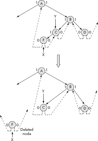
Fig. 7.47 Deletion of a left leaf node
CASE 2:
When X is a right leaf node, then its parent Y is found. The right child of Y is made to point where X’s right thread is currently pointing to. The RTag of Y is set to 0, indicating that it has become a thread now.
An algorithm for deletion of a node X which is a right leaf node is given below:
   Algorithm delRightLeaf (X,Y)
   {
     Y = findParent (X);
     if (rightChild (Y) == X)
     {
      rightChild (Y) = rightChild (X);   /* Make right child of parent as    thread
                                         and let it point where X’s left thread is
                                         pointing */
      RTag (Y) = 0;
     }
     return X;
   }
This case is similar to CASE 1 and, therefore, illustration for this case is not provided.
CASE 3:
When X is having a right sub-tree, its parent Y is found. A pointer called ‘grandson’ is make to point to the right child of X (see fig 7.48). The right child of Y is pointed to grandson. The successor of X is found. The left thread of successor is pointed to Y, indicating that the successor of X has now become the successor of parent as shown in Figure 7.48.
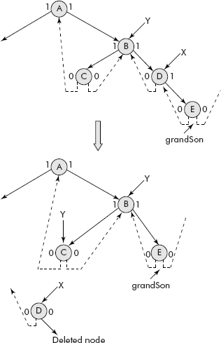
Fig. 7.48 Deletion of a node having only right sub-tree
It may be noted that in Figure 7.48, the grandson is also the successor of X.
An algorithm for deletion of X when X is having a right sub-tree is given below:
   Algorithm delNonLeafR (X, Y)
   {
     Y = findParent (X);
     if (RTag (X) == 1)
   {
     grandson = rightChild (X);
     rightChild (Y) = grandson;
     succ = inOrderSucc(X);
     leftChild (succ) = Y;
   }
   return X
  }
CASE 4:
When X is having only left sub-tree, its parent Y is found. A pointer called ‘grandson’ is made to point to the left child of X. The left child of Y is pointed to grandson. The predecessor of X is found. The right thread of predecessor is pointed to Y, indicating that the predecessor of X has now become the predecessor of parent.
An algorithm for deletion of X when X is having a left sub-tree is given below:
   Algorithm delNonLeafL (X, Y)
   {
    Y = findParent (X);
    if (LTag (X) == 1)
    {
     grandson = leftChild (X);
     leftChild (Y) = grandson;
     pred = inOrderPred(X);
     rightChild (pred) = Y;
    }
    return X
   }
This case is similar to CASE 3 and, therefore, illustration for this case is not provided.
CASE 5:
When X is having both sub-trees, then X is not deleted but its successor is found. The data of successor is copied in X and the successor is deleted using either CASE 1 or CASE 2, whichever is applicable.
An algorithm for deletion of X when X is having both sub-trees is given below:
   Algorithm delBoth (X)
   {
     succ = findSucc (X);
     DATA (X) = DATA (succ);
     Delete succ using Case1 or Case2
   }
Note: The applications of threaded binary trees are limited in the sense that the above discussions per-tain to inorder threaded binary trees only. For postorder, the above algorithms need to be rewritten. The implementation is rather complex.
EXERCISES
- What is the need of tree data structure? Explain with the help of examples. List out the areas in which this data structure can be applied extensively.
- What is a tree? Discuss why definition of tree is recursive. Why it is said to be non-linear?
- Define the following terms:
- Root
- Empty tree
- Leaf nodes
- Sub-tree
- Discuss the following terms with suitable examples:
- Parent
- Child
- Sibling
- Internal node
- Edge
- Path
- Depth
- Height
- Degree
- Explain binary tree with the help of examples. Discuss the properties of binary tree that need to be considered.
- Discuss the concept of full binary tree and complete binary tree. Differentiate between the two types with the help of examples.
- Discuss various methods of representation of a binary tree along with their advantages and disadvantages.
- Present an algorithm for creation of a binary tree. Consider a suitable binary tree to be created and discuss how the algorithm can be applied to create the required tree.
- What do you mean by tree traversal? What kinds of operations are possible on a node of a binary tree? Give an algorithm for inorder traversal of a binary tree. Taking an example, discuss how the binary tree can be traversed using inorder traversal.
- What do you mean by preorder traversal of a tree? Discuss an algorithm for preorder traversal of a binary tree along with an example.
- Give an algorithm for postorder traversal of a binary tree. Taking an example, discuss how the binary tree can be traversed using postorder traversal.
- What are the various types of binary trees?
- What is an expression tree? Consider the following preorder arithmetic expressions:
- + * − A B C D
- + A + B C
- / − A B C
- / * A + B C D
- + * A B / C D
- * A + B / C D
Draw expression tree for the above arithmetic expressions. Give the inorder, preorder and postorder traversal of the expression trees obtained.
- What is a binary search tree? What are the conditions applied on a binary tree to obtain a binary search tree? Present an algorithm to construct a binary search tree and discuss it using a suitable example.
- Discuss various operations that can be applied on a BST. Present an algorithm that searches a key in a BST. Take a suitable binary tree and search for a particular key in the tree by applying the discussed algorithm.
- Discuss how the insert operation can be performed in a binary tree with the help of an algorithm. Consider a binary tree and insert a particular value in the binary tree.
- Discuss how the delete operation can be performed in a binary tree. Also, present an algorithm for the same. Consider a binary tree and delete a particular value in the binary tree.
- Discuss the process of deletion of a node in a binary tree for the following cases by taking suitable examples:
- The node is a leaf node.
- The node has only one child.
- The node is an internal node, i.e., has both the children.
- What are heap trees? Discuss representation of a heap tree. Discuss a minheap tree and a maxheap tree with the help of examples. What are the operations that can be performed on a heap tree?
- Discuss insertion and deletion of a node into/from a heap tree using examples. Present an algorithm for both the operations.
- Consider the BST shown in Figure 7.49:
Perform the following operations on the above BST:
- Search a given key, say 7, in the BST:.
- Insert a given key, say 10, in the BST.
- Insert a given key, say 52, in the BST.
- Delete a given key, say 11, in the BST.
- Delete a given key, say 10, in the BST.
- Delete a given key, say 1, in the BST.
Display appropriate messages.
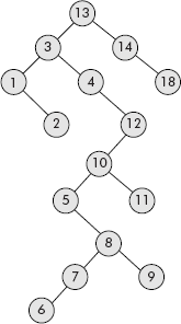
Fig. 7.49 A binary search tree of Q.21
- Consider the following list of numbers input by the user:
12, 5, 18, 90, 43, 36, 81, 10, 15, 8, 23
- Construct a BST for the above list of non-negative integers.
- Search a given key, say 43, in the BST created.
- Search a given key, say 93, in the BST created.
- Insert a given key, say 48, in the BST created.
- Insert a given key, say 23, in the BST created.
- Delete 23 from the above BST created.
- Delete 5 from the above BST created.
- Delete 12 from the above BST created.
Display appropriate messages.
- What do you mean by sorting? Discuss heap sort in detail with the help of an example.
- Consider the maxheap shown in Figure 7.50. Perform the desired operations on the heap to obtain a sorted list of elements. Display the sorted list obtained.
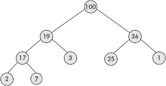
Fig. 7.50 Maxheap of Q.24