Chapter 7. Machine Learning for Microscopy
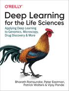
In this chapter, we introduce you to deep learning techniques for microscopy. In such applications, we seek to understand the biological structure of a microscopic image. For example, we might be interested in counting the number of cells of a particular type in a given image, or we might seek to identify particular organelles. Microscopy is one of the most fundamental tools for the life sciences, and advances in microscopy have greatly advanced human science. Seeing is believing even for skeptical scientists, and being able to visually inspect biological entities such as cells builds an intuitive understanding of the underlying mechanisms of life. A vibrant visualization of cell nuclei and cytoskeletons (as in Figure 7-1) builds a much deeper understanding than a dry discussion in a textbook.
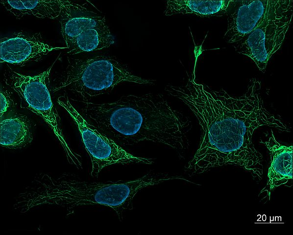
Figure 7-1. Human-derived SK8/18-2 cells. These cells are stained to highlight their nuclei and cytoskeletons and imaged using fluorescence microscopy. (Source: Wikimedia.)
.jpg)
The question remains how deep learning can make a difference in microscopy. Until recently, the only way to analyze microscopy images was to have humans (often graduate students or research associates) manually inspect these images for useful patterns. More recently, tools such as CellProfiler have made it possible for biologists to automatically assemble pipelines for handling imaging data.
Automated High-Throughput Microscopy Image Analysis
Advances in automation in the last few decades have made it feasible to perform automated high-throughput microscopy on some systems. These systems use a combination of simple robotics (for automated handling of samples) and image processing algorithms to automatically process images. These image processing applications such as separating the foreground and background of cells and obtaining simple cell counts and other basic measurements. In addition, tools like CellProfiler have allowed biologists without programming experience to construct new automated pipelines for handling cellular data.
However, automated microscopy systems have traditionally faced a number of limitations. For one, complex visual tasks couldn’t be performed by existing computer vision pipelines. In addition, properly preparing samples for analysis takes considerable sophistication on the part of the scientist running the experiment. For these reasons, automated microscopy has remained a relatively niche technique, despite its considerable success in enabling sophisticated new experiments.
Deep learning consequently holds considerable promise for extending the capabilities of tools such as CellProfiler. If deep analysis methods can perform more complex analyses, automated microscopy could become a considerably more effective tool. For this reason, there has been considerable research interest in deep microscopy, as we shall see in the remainder of this chapter.
The hope of deep learning techniques is that they will enable automated microscopy pipelines to become significantly more flexible. Deep learning systems show promise at being able to perform nearly any task a human image analyst can. In addition, early research suggests that deep learning techniques could considerably expand the capabilities of inexpensive microscopy hardware, potentially allowing cheap microscopes to perform analyses currently possible only using very sophisticated and expensive apparatuses.
Looking forward, it is even possible to train deep models that “simulate” experimental assays. Such systems are capable of predicting the outcomes of experiments (in some limited cases) without even running the experiment in question. This is a very powerful capability, and one which has spurred much excitement about the potential for deep networks in image-based biology.
In this chapter, we will teach you the basics of deep microscopy. We will demonstrate how deep learning systems can learn to perform simple tasks such as cell counting and cellular segmentation. In addition, we will discuss how to build extensible systems that could serve to handle more sophisticated image processing pipelines.
A Brief Introduction to Microscopy
Before we dive into algorithms, let’s first talk basics. Microscopy is the science of using physical systems to view small objects. Traditionally, microscopes were purely optical devices, using finely ground lenses to expand the resolution of samples. More recently, the field of microscopy has started to lean heavily on technologies such as electron beams or even physical probes to produce high-resolution samples.
Microscopy has been tied intimately to the life sciences for centuries. In the 17th century, Anton van Leeuwenhoek used early optical microscopes (of his own design and construction) to describe microorganisms in unprecedented detail (as shown in Figure 7-2). These observations depended critically on van Leeuwenhoek’s advances in microscopy, and in particular on his invention of a new lens which allowed for significantly improved resolution over the microscopes available at the time.
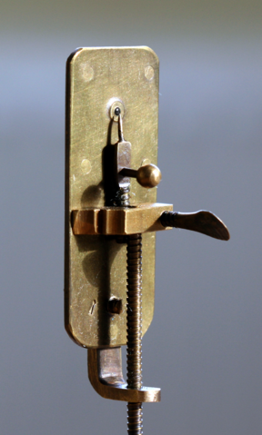
Figure 7-2. A reproduction of van Leeuwenhoek’s microscope constructed in the modern era. Van Leeuwenhoek kept key details of his lens grinding process private, and a successful reproduction of the microscope wasn’t achieved until the 1950s by scientists in the United States and the Soviet Union. (Source: Wikimedia.)
The invention of high-resolution optical microscopes triggered a revolution in microbiology. The spread of microscopy techniques and the ability to view cells, bacteria, and other microorganisms at scale enabled the entire field of microbiology and the pathogenic model of disease. It’s hard to overstate the effect of microscopy on the modern life sciences.
Optical microscopes are either simple or compound. Simple microscopes use only a single lens for magnification. Compound microscopes use multiple lenses to achieve higher resolution, but at the cost of additional complexity in construction. The first practical compound microscopes weren’t achieved until the middle of the 19th century! Arguably, the next major shift in optical microscopy system design didn’t happen until the 1980s, with the advent of digital microscopes, which enabled the images captured by a microscope to be written to computer storage. As we mentioned in the previous section, automated microscopy uses digital microscopes to capture large volumes of images. These can be used to conduct large-scale biological experiments that capture the effects of experimental perturbations.
Modern Optical Microscopy
Despite the fact that optical microscopy has been around for centuries, there’s still considerable innovation happening in the field. One of the most fundamental techniques is optical sectioning. An optical microscope has focal planes where the microscope is currently focused. A variety of techniques to focus the image on a chosen focal plane have been developed. These focused images can then be stitched together algorithmically to create a high-resolution image or even a 3D reconstruction of the original image. Figure 7-3 visually demonstrates how sectioned images of a grain of pollen can be combined to yield a high-fidelity image.
Confocal microscopes are a common solution to the problem of optical sectioning. They use a pinhole to block light coming in from out of focus, allowing a confocal microscope to achieve better depth perception. By shifting the focus of the microscope and doing a horizontal scan, you can get a full picture of the entire sample with increased optical resolution and contrast. In an interesting historical aside, the concept of confocal imaging was first patented by the AI pioneer Marvin Minsky (see Figure 7-4).
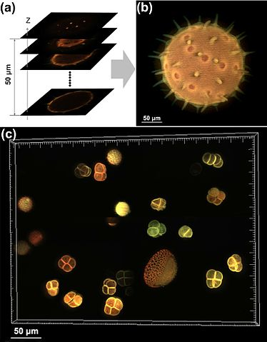
Figure 7-3. Pollen grain imaging: (a) optically sectioned fluorescence images of a pollen grain; (b) combined image; (c) combined image of a group of pollen grains. (Source: Wikimedia.)
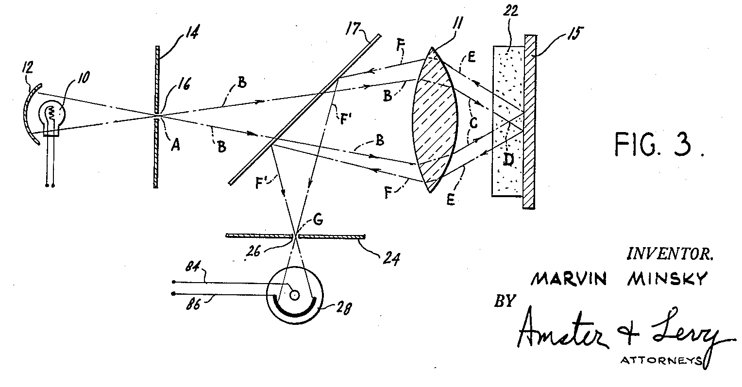
Figure 7-4. An image from Minsky’s original patent introducing a confocal scanning microscope. In a curious twist of history, Minsky is better known for his pioneering work in AI. (Source: Wikimedia.)
Well-designed optical sectioning microscopes excel at capturing 3D images of biological systems since scans can be used to focus on multiple parts of the image. These focused images can be stitched together algorithmically, yielding beautiful 3D reconstructions.
In the next section, we will explore some of the fundamental limits that constrain optical microscopy and survey some of the techniques that have been designed to work around these limitations. This material isn’t directly related to deep learning yet (for reasons we shall discuss), but we think it will give you a valuable understanding of the challenges facing microscopy today. This intuition will prove useful if you want to help design the next generation of machine learning–powered microscopy systems. However, if you’re in a hurry to get to some code, we encourage you to skip forward to the subsequent sections where we dive into more immediate applications.
What Can Deep Learning Not Do?
It seems intuitively obvious that deep learning can make an impact in microscopy, since deep learning excels at image handling and microscopy is all about image capture. But it’s worth asking: what parts of microscopy can’t deep learning do much for now? As we see later in this chapter, preparing a sample for microscopic imaging can require considerable sophistication. In addition, sample preparation requires considerable physical dexterity, because the experimenter must be capable of fixing the sample as a physical object. How could we possibly automate or speed up this process with deep learning?
The unfortunate truth right now is that robotic systems are still very limited. While simple tasks like confocal scans of a sample are easy to handle, cleaning and preparing a sample requires considerable expertise. It’s unlikely that any robotic systems available in the near future will have this ability.
Whenever you hear forecasts about the future impact of learning techniques, it’s useful to keep examples like sample preparation in mind. Many of the pain points in the life sciences involve tasks such as sample preparation that just aren’t feasible for today’s machine learning. That may well change, but likely not for the next few years at the least.
The Diffraction Limit
When studying a new physical instrument such as a microscope, it can be useful to start by trying to understand its limits. What can’t microscopes do? It turns out this question has been studied in great depth by previous generations of physicists (with some recent surprises too!). The first place to start is the diffraction limit, a theoretical limit on the resolution possible with a microscope:
The quantity is often rewritten as the numerical aperture, NA. is the wavelength of light. Note the implicit assumptions here. We assume that the sample is illuminated with some form of light. Let’s take a quick look at the spectrum of light waves out there (see Figure 7-5).
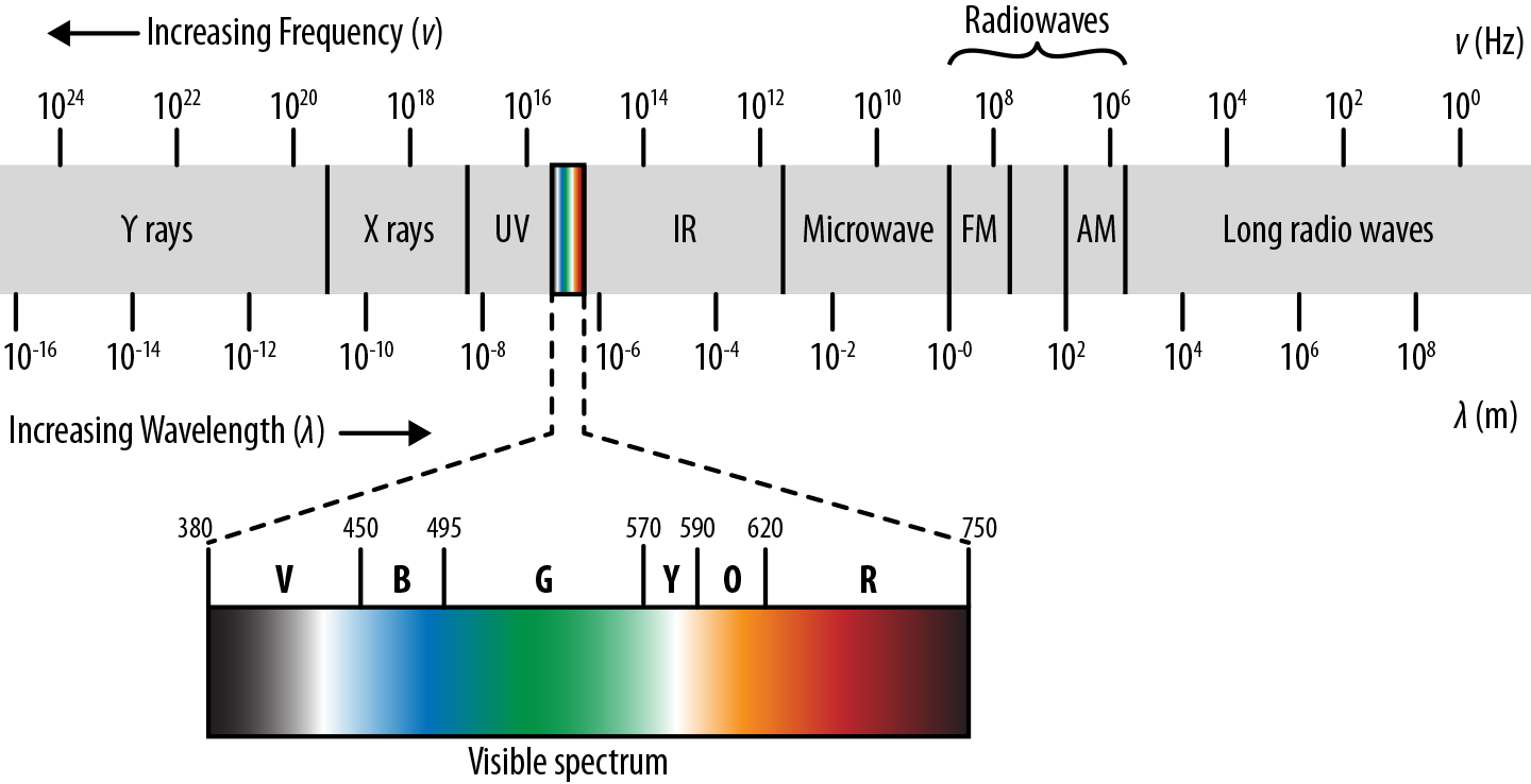
Figure 7-5. Wavelengths of light. Note that low-wavelength light sources such as X-rays are increasingly energetic. As a result, they will often destroy delicate biological samples.
Note how visible light forms only a tiny fraction of this spectrum. In principle, we should be able to make the desired resolution arbitrarily good using light at a low enough wavelength. To some extent this has happened already. A number of microscopes use electromagnetic waves of higher energy. For example, ultraviolet microscopes use the fact that UV rays have smaller wavelengths to allow for higher resolution. Couldn’t we take this pattern further and use light of even smaller wavelength? For example, why not an X-ray or gamma-ray microscope? The main issue here is phototoxicity. Light with small wavelengths is highly energetic. Shining such light upon a sample can destroy the structure of the sample. In addition, high-wavelength light is dangerous for the experimenter and requires special experimental facilities.
Luckily, though, there exist a number of other techniques for bypassing the diffraction limit. One uses electrons (which have wavelengths too!) to image samples. Another uses physical probes instead of light. Yet another method for avoiding the resolution limit is to make use of near-field electromagnetic waves. Tricks with multiple illuminated fluorophores can also allow the limit to be lowered. We’ll discuss these techniques in the following sections.
Electron and Atomic Force Microscopy
In the 1930s, the advent of the electron microscope triggered a dramatic leap in modern microscopy. The electron microscope uses electron beams instead of visible light in order to obtain images of objects. Since the wavelengths of electrons are much smaller than those of visible light, using electron beams instead of light waves allows much more detailed images. Why does this make any sense? Well, aren’t electrons particles? Remember that matter can exhibit wave-like properties. This is known as the de Broglie wavelength, which was first proposed by Louis de Broglie:
Here, is Planck’s constant and and are the mass and velocity of the particle in question. (For the physicists, note that this formula doesn’t account for relativistic effects. There are modified versions of the formula that do so.) Electron microscopes make use of the wave-like nature of electrons to image physical objects. The wavelength of an electron depends on its energy, but is easily subnanometer at wavelengths achievable by a standard electron gun. Plugging into the diffraction limit model discussed previously, it’s easy to see how electron microscopy can be a powerful tool. The first prototype electron microscopes were constructed in the early 1930s. While these constructions have been considerably refined, today’s electron microscopes still depend on the same core principles (see Figure 7-6).
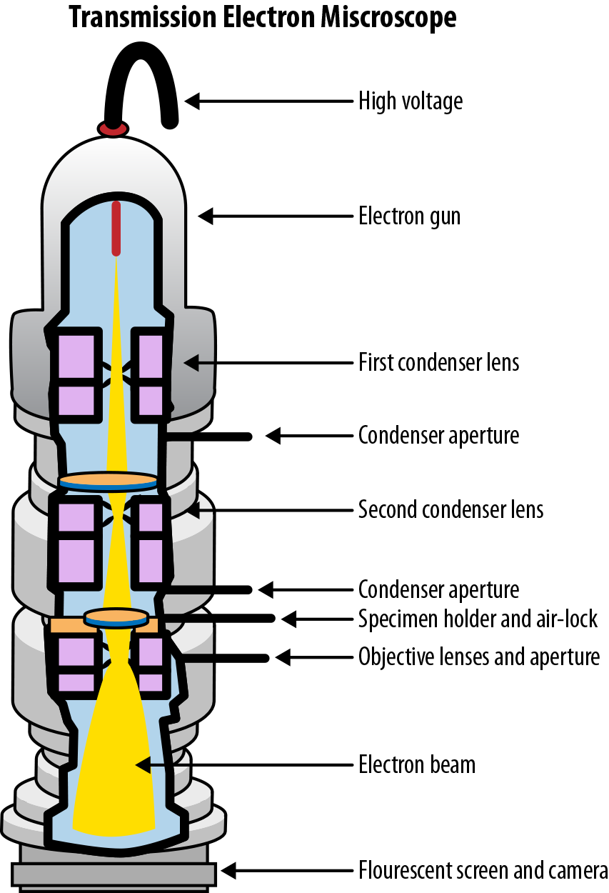
Figure 7-6. The components of a modern transmission electron microscope. (Source: Wikimedia.)
Note that we haven’t entirely bypassed the issues with phototoxicity here. To get electrons with very small wavelengths, we need to increase their energy—and at very high energy, we will again destroy samples. In addition, the process of preparing samples for imaging by an electron microscope can be quite involved. Nevertheless, the use of electron microscopes has allowed for stunning images of microscopic systems (see Figure 7-7). Scanning electron microscopes, which scan the input sample to achieve larger fields of view,allow for images with resolution as small as one nanometer.
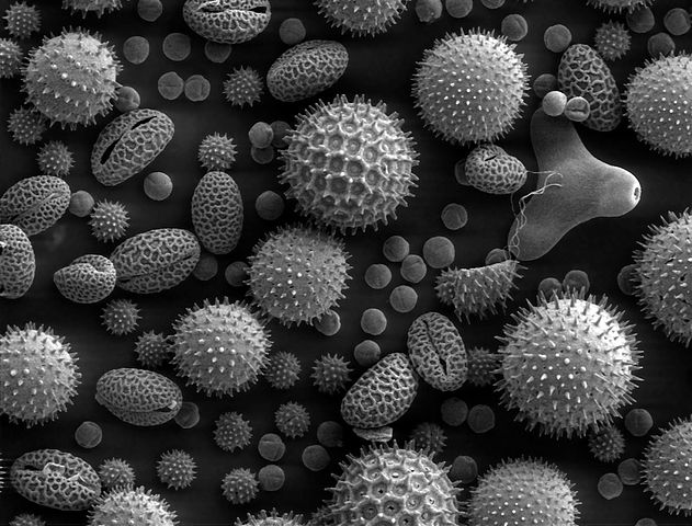
Figure 7-7. Pollen magnified 500x by a scanning electron microscope. (Source: Wikimedia.)
Atomic force microscopy (AFM) provides another way of breaking through the optical diffraction limit. This technique leverages a cantilever which probes a given surface physically. The direct physical contact between the cantilever and the sample allows for pictures with resolutions at fractions of a nanometer. Indeed, it is sometimes possible to image single atoms! Atomic force microscopes also provide for 3D images of a surface due to the direct contact of the cantilever with the surface at hand.
Force microscopy broadly is a recent technique. The first atomic force microscopes were only invented in the 1980s, after nanoscale manufacturing techniques had matured to a point where the probes involved could be accurately made. As a result, applications in the life sciences are still emergent. There has been some work on imaging cells and biomolecules with AFM probes, but these techniques are still early.
Super-Resolution Microscopy
We’ve discussed a number of ways to stretch the diffraction limit so far in this chapter, including using higher-wavelength light or physical probes to allow for greater resolution. However, in the second half of the 20th century came a scientific breakthrough, led by the realization that there existed entire families of methods for breaking past the diffraction limit. Collectively, these techniques are called super-resolution microscopy techniques:
- Functional super-resolution microscopy
-
Makes use of physical properties of light-emitting substances embedded in the sample being imaged. For example, fluorescent tags (more on these later) in biological microscopy can highlight particular biological molecules. These techniques allow standard optical microscopes to detect light emitters. Functional super-resolution techniques can be broadly split into deterministic and stochastic techniques.
- Deterministic super-resolution microscopy
-
Some light-emitting substances have a nonlinear response to excitation. What does this actually mean? The idea is that arbitrary focus on a particular light emitter can be achieved by “turning off” the other emitters nearby. The physics behind this is a little tricky, but well-developed techniques such as stimulated emission depletion (STED) microscopy have demonstrated this technique.
- Stochastic super-resolution microscopy
-
Light-emitting molecules in biological systems are subject to random motion. This means that if the motion of a light-emitting particle is tracked over time, its measurements can be averaged to yield a low error estimate of its true position. There are a number of techniques (such as STORM, PALM, and BALM microscopy) that refine this basic idea. These super-resolution techniques have had a dramatic effect in modern biology and chemistry because they allow relatively cheap optical equipment to probe the behavior of nanoscale systems. The 2014 Nobel Prize in Chemistry was awarded to pioneers of functional super-resolution techniques.
Deep Super-Resolution Techniques
Recent research has started to leverage the power of deep learning techniques to reconstruct super-resolution views.1 These techniques claim orders of magnitude improvements in the speed of super-resolution microscopy by enabling reconstructions from sparse, rapidly acquired images. While still in its infancy, this shows promise as a future application area for deep learning.
Near-field microscopy is another super-resolution technique that makes use of local electromagnetic information in a sample. These “evanescent waves” don’t obey the diffraction limit, so higher resolution is possible. However, the trade-off is that the microscope has to gather light from extremely close to the sample (within one wavelength of light from the sample). This means that although near-field techniques make for extremely interesting physics, practical use remains challenging. Very recently, it has also become possible to construct “metamaterials” which have a negative refractive index. In effect, the properties of these materials mean that near-field evanescent waves can be amplified to allow imaging further away from the sample. Research in this field is still early but very exciting.
Deep Learning and the Diffraction Limit?
Tantalizing hints suggest that deep learning may facilitate the spread of super-resolution microscopy. A few early papers have shown that it might be possible for deep learning algorithms to speed up the construction of super-resolution images or enable effective super-resolution with relatively cheap hardware. (We point to one such paper in the previous note.)
These hints are particularly compelling because deep learning can effectively perform tasks such as image deblurring.2 This evidence suggests that it may be possible to build a robust set of super-resolution tools based on deep learning that could dramatically facilitate the adoption of such techniques. At present this research is still immature, and compelling tooling doesn’t yet exist. However, we hope that this state of affairs will change over the coming years.
Preparing Biological Samples for Microscopy
One of the most critical steps in applying microscopy in the life sciences is preparing the sample for the microscope. This can be a highly nontrivial process that requires considerable experimental sophistication. We discuss a number of techniques for preparing samples in this section and comment on the ways in which such techniques can go wrong and create unexpected experimental artifacts.
Staining
The earliest optical microscopes allowed for magnified views of microscopic objects. This power enabled amazing improvements in the understanding of small objects, but it had the major limitation that it was not possible to highlight certain areas of the image for contrast. This led to the development of chemical stains which permitted scientists to view regions of the image for contrast.
A wide variety of stains have been developed to handle different types of samples. The staining procedures themselves can be quite involved, with multiple steps. Stains can be extraordinarily influential scientifically. In fact, it’s common to classify to bacteria as “gram-positive” or “gram-negative” depending on their response to the well known Gram stain for bacteria. A task for a deep learning system might be to segment and label the gram-positive and gram-negative bacteria in microscopy samples. If you had a potential antibiotic in development, this would enable you to study its effect on gram-positive and gram-negative species separately.
Why Should I Care as a Developer?
Some of you reading this section may be developers interested in dealing with the challenges of building and deploying deep microscopy pipelines. You might reasonably be asking yourself whether you should care about the biology of sample preparation.
If you are indeed laser-focused on the challenges of building pipelines, skipping ahead to the case studies in this chapter will probably help you most. However, building an understanding of basic sample preparation may save you headaches later on and give you the vocabulary to effectively communicate with your biologist peers. If biology requests that you add metadata fields for stains, this section will give you a good idea of what they’re actually asking for. That’s worth a few minutes of your time!
Developing Antibacterial Agents for Gram-Negative Bacteria
One of the major challenges in drug discovery at this time is developing effective antibiotics for gram-negative bacteria. Gram-negative bacteria have an additional cell wall that prevents common antibacterial agents which target the peptidoglycan cell walls of gram-positive bacteria from functioning effectively.
This challenge is becoming more urgent because many bacterial strains are picking up gram-negative resistance through methods such as horizontal gene transfer, and deaths from bacterial infections are once again on the rise after decades of control.
It might well be possible to combine the deep learning methods for molecular design you’ve seen already with some of the imaging-based techniques you’ll learn in this chapter to make progress on this problem. We encourage those of you curious about the possibilities to explore this area more carefully.
Sample Fixation
Large biological samples such as tissue will often degrade rapidly if left to their own devices. Metabolic processes in the sample will consume and damage the structure of the organs, cells, and organelles in the sample. The process of “fixation” seeks to stop this process, and stabilize the contents of the sample so that it can be imaged properly. A number of fixative agents have been designed which aid in this process. One of the core functions of fixatives is to denature proteins and turn off proteolytic enzymes. Such enzymes will consume the sample if allowed.
In addition, the process of fixation seeks to kill microorganisms that may damage the sample. For example, in heat fixation the sample is passed through a Bunsen burner. This process can damage the internal structures of the sample as a side effect. Another common technique is that of immersion fixation, where samples are immersed in a fixative solution and allowed to soak. For example, a sample could be soaked in cold formalin for a span of time, such as 24 hours.
Perfusion is a technique for fixing tissue samples from larger animals such as mice. Experimenters inject fixative into the heart and wait for the mouse to die before extracting the tissue sample. This process allows for the fixative agent to spread through the tissue naturally and often yields superior results.
Sectioning Samples
An important part of viewing a biological sample is being able to slice out a thin part of the sample for the microscope. There exist a number of ingenious tools to facilitate this process, including the microtome (see Figure 7-8), which slices biological samples into thin slices for easy viewing. The microtome has its limitations: it’s hard to slice very small objects this way. For such small objects, it might be better to use a technique such as confocal microscopy instead.
It’s worth pausing and asking why it’s useful to know that devices such as a microtome exist. Well, let’s say that as an engineer, you’re constructing a pipeline to handle a number of brain imaging samples. The sample brain was likely sliced into thin pieces using a microtome or similar cutting device. Knowing the physical nature of this process will aid you if you’re (for example) building a schema to organize such images consistently.
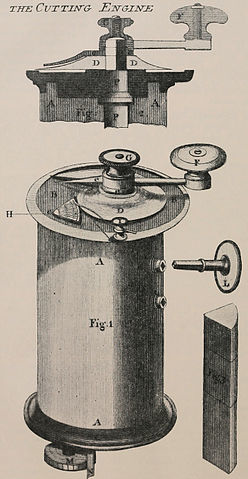
Figure 7-8. An early diagram from 1770 depicting a microtome. (Source: Wikimedia.)
Fluorescence Microscopy
A fluorescence microscope is an optical microscope that makes use of the phenomenon of fluorescence, where a sample of material absorbs light at one wavelength and emits it at another wavelength. This is a natural physical phenomenon; for example, a number of minerals fluoresce when exposed to ultraviolet light. It gets particularly interesting when applied to biology, though. A number of bacteria fluoresce naturally when their proteins absorb high-energy light and emit lower-energy light.
Fluorophores and fluorescent tags
A fluorophore is a chemical compound that can reemit light at a certain wavelength. These compounds are a critical tool in biology because they allow experimentalists to image particular components of a given cell in detail. Experimentally, the fluorophore is commonly applied as a dye to a particular cell. Figure 7-9 shows the molecular structure of a common fluorophore.
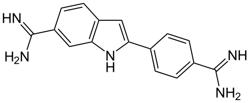
Figure 7-9. DAPI (4',6-diamidino-2-phenylindole) is a common fluorescent stain that binds to adenine-thymine–rich regions of DNA. Because it passes through cell membranes, it is commonly used to stain the insides of cells. (Source: Wikimedia.)
Fluorescent tagging is a technique for attaching a fluorophore to a biomolecule of interest in the body. There are a variety of techniques to do this effectively. It’s useful in microscopy imaging, where it’s common to want to highlight a particular part of the image. Fluorescent tagging can enable this very effectively.
Fluorescent microscopy has proven a tremendous boon for biological research because it permits researchers to zoom in on specific subsystems in a given biological sample, as opposed to dealing with the entirety of the sample. When studying individual cells, or individual molecules within a cell, the use of tagging can prove invaluable for focusing attention on interesting subsystems. Figure 7-10 shows how a fluorescent stain can be used to selectively visualize particular chromosomes within a human cell nucleus.
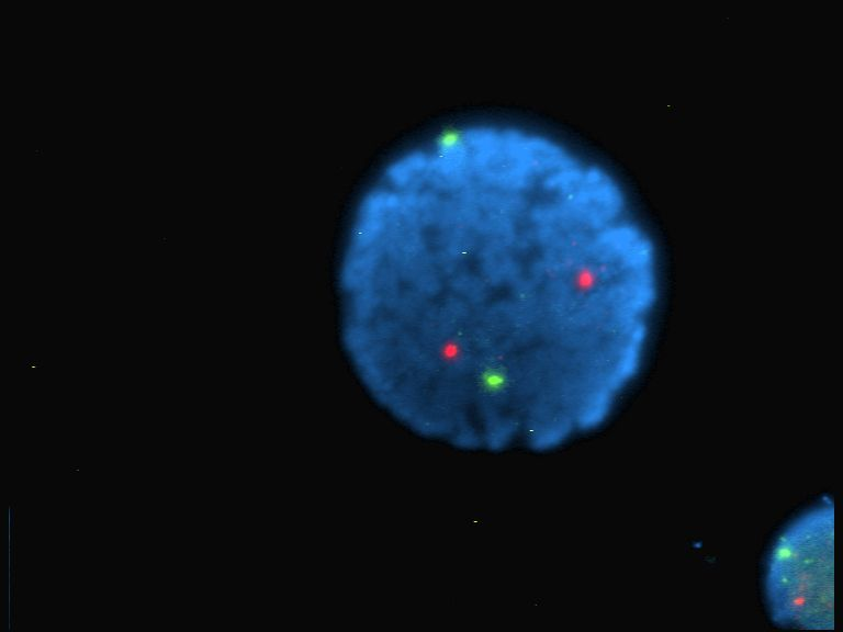
Figure 7-10. An image of a human lymphocyte nucleus with chromosomes 13 and 21 stained with DAPI (a popular fluorescent stain) to emit light. (Source: Wikimedia.)
Fluorescence microscopy can be a very precise tool, used to track events like single binding events of molecules. For example, binding events of proteins to ligands (as discussed in Chapter 5) can be detected by a fluorescence assay.
Sample Preparation Artifacts
It’s important to note that sample preparation can be a deeply tricky process. It’s common for the preparation of the original sample to induce distortions in the object being imaged, which can lead to some confusion. An interesting example is the case of the mesosome, discussed in the following warning note.
The Mesosome: An Imaginary Organelle
The process of fixing a cell for electron microscopy introduces a crucial artifact, the mesosome in gram-positive bacteria (see Figure 7-11). Degradations in the cell wall, caused by the process of preparing the sample for the electron microscope, were originally thought to be natural structures instead of artifacts.
Be warned that similar artifacts likely exist in your own samples. In addition, it’s entirely possible that a deep network could train itself to detect such artifacts rather than training itself to find real biology.
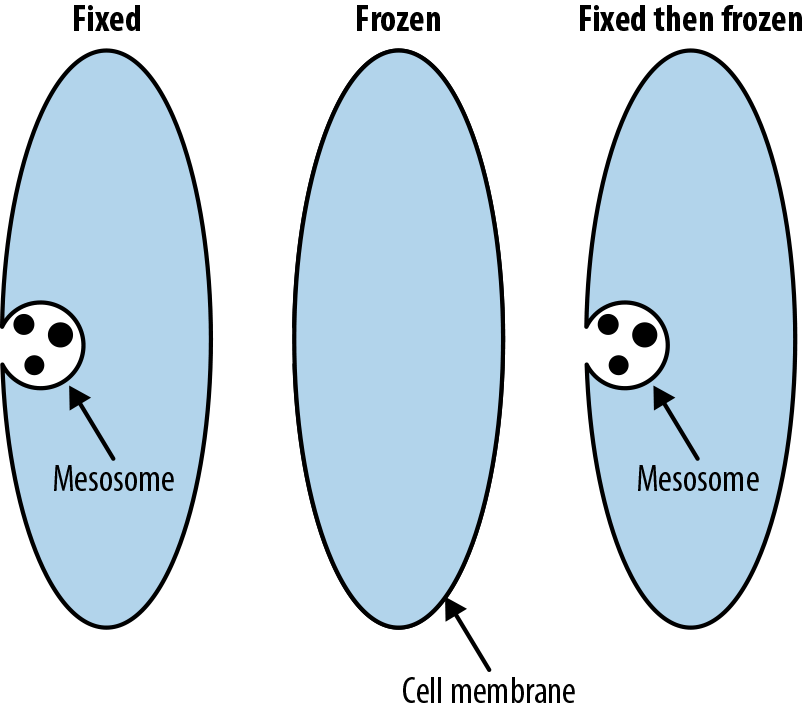
Figure 7-11. Mesosomes are artifacts introduced by preparation for electron microscopy that were once believed to be real structures in cells. (Adapted from Wikimedia.)
Tracking Provenance of Microscopy Samples
When you’re designing systems to handle microscopy data, it will be critical to track the provenance of your samples. Each image should be annotated with information about the conditions in which it was gathered. This might include the physical device that was used to capture the image, the technician who supervised the imaging process, the sample that was imaged, and the physical location at which the sample was gathered. Biology is extraordinarily tricky to “debug.” Issues such as the one described in the previous warning can go untracked, potentially for decades. Making sure to maintain adequate metadata around the provenance of your images could save you and your team from major issues down the line.
Deep Learning Applications
In this section we briefly review various applications of deep learning to microscopy, such as cell counting, cell segmentation, and computational assay construction. As we’ve noted previously in the chapter, this is a limited subset of the applications possible for deep microscopy. However, understanding these basic applications will give you the understanding needed to invent new deep microscopy applications of your own.
Cell Counting
A simple task is to count the number of cells that appear in a given image. You might reasonably ask why this is an interesting task. For a number of biological experiments, it can be quite useful to track the number of cells that survive after a given intervention. For example, perhaps the cells are drawn from a cancer cell line, and the intervention is the application of an anticancer compound. A successful intervention would reduce the number of living cancer cells, so it would be useful to have a deep learning system that can count the number of such living cells accurately without human intervention.
What Is a Cell Line?
Often in biology, it’s useful to study cells of a given type. The first step in running an experiment against a collection of cells is to gain a plentiful supply of such cells. Enter the cell line. Cell lines are cells cultivated from a given source and that can grow stably in laboratory conditions.
Cell lines have been used in countless biological papers, but there are often serious concerns about the science done on them. To start, removing a cell from its natural environment can radically change its biology. A growing line of evidence shows that the environment of a cell can fundamentally shape its response to stimuli.
Even more seriously, cell lines are often contaminated. Cells from one cell line may contaminate cells from another cell line, so results on a “breast cancer” cell line may, in fact, tell the researcher absolutely nothing about breast cancer!
For these reasons, studies on cell lines are often treated with caution, with the results intended simply as spur to attempt duplication with animal or human tests. Nevertheless, cell line studies provide an invaluable easy entry point to biological research and remain ubiquitous.
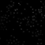
Figure 7-12. Samples of Drosophila cells. Note how the image conditions in microscopy images can be significantly different from image conditions in photographs. (Source: Cell Image Library.)
As Figure 7-12 shows, image conditions in cell microscopy can be significantly different from standard image conditions, so it is not immediately obvious that technologies such as convolutional neural networks can be adapted to tasks such as cell counting. Luckily, significant experimental work has shown that convolutional networks do quite well at learning from microscopy datasets.
Implementing cell counting in DeepChem
This section walks through the construction of a deep learning model for cell counting using DeepChem. We’ll start by loading and featurizing a cell counting dataset. We use the Broad Bioimage Benchmark Collection (BBBC) to get access to a useful microscopy dataset for this purpose.
BBBC Datasets
The BBBC datasets contain a useful collection of annotated bioimage datasets from various cellular assays. It is a useful resource as you work on training your own deep microscopy models. DeepChem has a collection of image processing resources to make it easier to work with these datasets. In particular, DeepChem’s ImageLoader class facilitates loading of the datasets.
Processing Image Datasets
Images are usually stored on disk in standard image file formats (PNG, JPEG, etc.). The processing pipeline for image datasets typically reads in these files from disk and transforms them into a suitable in-memory representation, typically a multidimensional array. In Python processing pipelines, this array is often simply a NumPy array. For an image N pixels high, M pixels wide, and with 3 RGB color channels, you would get an array of shape (N, M, 3). If you have 10 such images, these images would typically be batched into an array of shape (10, N, M, 3).
Before you can load the dataset into DeepChem, you’ll first need to download it locally. The BBBC005 dataset that we’ll use for this task is reasonably large (a little under 2 GB), so make sure your development machine has sufficient space available:
wget https://data.broadinstitute.org/bbbc/BBBC005/BBBC005_v1_images.zip
unzip BBBC005_v1_images.zip
With the dataset downloaded to your local machine, you can now load this dataset into DeepChem by using ImageLoader:
image_dir='BBBC005_v1_images'files=[]labels=[]forfinos.listdir(image_dir):iff.endswith('.TIF'):files.append(os.path.join(image_dir,f))labels.append(int(re.findall('_C(.*?)_',f)[0]))loader=dc.data.ImageLoader()dataset=loader.featurize(files,np.array(labels))
This code walks through the downloaded directory of images and pulls out the image files. The labels are encoded in the filenames themselves, so we use a simple regular expression to extract the number of cells in each image. We use ImageLoader to transform this into a DeepChem dataset.
Let’s now split this dataset into training, validation, and test sets:
splitter=dc.splits.RandomSplitter()train_dataset,valid_dataset,test_dataset=splitter.train_valid_test_split(dataset,seed=123)
With this split in place, we can now define the model itself. In this case, let’s make a simple convolutional architecture with a fully connected layer at the end:
learning_rate=dc.models.tensorgraph.optimizers.ExponentialDecay(0.001,0.9,250)model=dc.models.TensorGraph(learning_rate=learning_rate,model_dir='model')features=layers.Feature(shape=(None,520,696))labels=layers.Label(shape=(None,))prev_layer=featuresfornum_outputsin[16,32,64,128,256]:prev_layer=layers.Conv2D(num_outputs,kernel_size=5,stride=2,in_layers=prev_layer)output=layers.Dense(1,in_layers=layers.Flatten(prev_layer))model.add_output(output)loss=layers.ReduceSum(layers.L2Loss(in_layers=(output,labels)))model.set_loss(loss)
Note that we use L2Loss to train our model as a regression task. Even though cell counts are whole numbers, we don’t have a natural upper bound on the number of cells in an image.
Training this model will take some computational effort (more on this momentarily), so to start, we recommend using our pretrained model for basic experimentation. This model can be used to make predictions out of the box. There are directions on downloading the pretrained model in the code repository associated with the book. Once you’ve downloaded it, you can load the pretrained weights into the model with:
model.restore()
Let’s take this pretrained model out for a whirl. First, we’ll compute the average prediction error on our test set for our cell counting task:
y_pred=model.predict(test_dataset).flatten()(np.sqrt(np.mean((y_pred-test_dataset.y)**2)))
What accuracy do you get when you try running the model?
Now, how can you train this model for yourself? You can fit the model by training it for 50 epochs on the dataset:
model.fit(train_dataset,nb_epoch=50)
This learning task will take some amount of computing horsepower. On a good GPU, it should complete within an hour or so. It may not be feasible to easily train the model on a CPU system.
Once trained, test the accuracy of the model on the validation and test sets. Does it match that of the pretrained model?
Cell Segmentation
The task of cellular segmentation involves annotating a given cellular microscopy image to denote where cells appear and where background appears. Why is this useful? If you recall our earlier discussion of gram-positive and gram-negative bacteria, you can probably guess why an automated system for separating out the two types of bacteria might prove useful. It turns out that similar problems arise through all of cellular microscopy (and in other fields of imaging, as we will see in Chapter 8).
Segmentation masks provide significantly finer-grained resolution and permit for more refined analysis than cell counting. For example, it might be useful to understand what fraction of a given plate is covered with cells. Such analysis is easy to perform once segmentation masks have been generated. Figure 7-13 provides an example of a segmentation mask that is generated from a synthetic dataset.
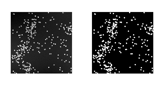
Figure 7-13. A synthetic dataset of cells (on the left) along with foreground/background masks annotating where cells appear in the image. (Source: Broad Institute.)
That said, segmentation asks for significantly more from a machine learning model than counting. Being able to precisely differentiate cellular and noncellular regions requires greater precision in learning. For that reason, it’s not surprising that machine learning segmentation approaches are still harder to get working than simpler cellular counting approaches. We will experiment with a segmentation model later in this chapter.
Where Do Segmentation Masks Come From?
It’s worth pausing to note that segmentation masks are complex objects. There don’t exist good algorithms (except for deep learning techniques) for generating such masks in general. How then can we bootstrap the training data needed to refine a deep segmentation technique? One possibility is to use synthetic data, as in Figure 7-13. Because the cellular image is generated in a synthetic fashion, the mask can also be synthetically generated. This is a useful trick, but it has obvious limitations because it will limit our learned segmentation methods to similar images.
A more general procedure is to have human annotators generate suitable segmentation masks. Similar procedures are used widely to train self-driving cars. In that task, finding segmentations that annotate pedestrians and street signs is critical, and armies of human segmenters are used to generate needed training data. As machine-learned microscopy grows in importance, it is likely that similar human pipelines will become critical.
Implementing cell segmentation in DeepChem
In this section, we will train a cellular segmentation model on the same BBBC005 dataset that we used previously for the cell counting task. There’s a crucial subtlety here, though. In the cell counting challenge, each training image has a simple count as a label. However, in the cellular segmentation task, each label is itself an image. This means that a cellular segmentation model is actually a form of “image transformer” rather than a simple classification or regression model. Let’s start by obtaining this dataset. We have to retrieve the segmentation masks from the BBBC website, using the following commands:
wget https://data.broadinstitute.org/bbbc/BBBC005/BBBC005_v1_ground_truth.zip
unzip BBBC005_v1_ground_truth.zip
The ground-truth data is something like 10 MB, so it should be easier to download than the full BBBC005 dataset. Now let’s load this dataset into DeepChem. Luckily for us, ImageLoader is set up to handle image segmentation datasets without much extra hassle:
image_dir='BBBC005_v1_images'label_dir='BBBC005_v1_ground_truth'rows=('A','B','C','D','E','F','G','H','I','J','K','L','M','N','O','P')blurs=(1,4,7,10,14,17,20,23,26,29,32,35,39,42,45,48)files=[]labels=[]forfinos.listdir(label_dir):iff.endswith('.TIF'):forrow,blurinzip(rows,blurs):fname=f.replace('_F1','_F%d'%blur).replace('_A','_%s'%row)files.append(os.path.join(image_dir,fname))labels.append(os.path.join(label_dir,f))loader=dc.data.ImageLoader()dataset=loader.featurize(files,labels)
Now that we have our datasets loaded and processed, let’s hop into building some deep learning models for them. As before, we’ll split this dataset into training, validation, and test sets:
splitter=dc.splits.RandomSplitter()train_dataset,valid_dataset,test_dataset=splitter.train_valid_test_split(dataset,seed=123)
What architecture can we use for the task of image segmentation? It’s not just a matter of using a straightforward convolutional architecture since our output needs to itself be an image (the segmentation mask). Luckily for us, there has been some past work on suitable architectures for this task. The U-Net architecture uses a stacked series of convolutions to progressively “downsample” and then “upsample” the source image, as illustrated in Figure 7-14. This architecture does well at the task of image segmentation.
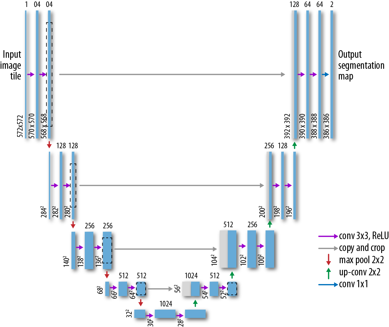
Figure 7-14. A representation of the U-Net architecture for biomedical image segmentation. (Adapted from the University of Freiburg.)
Let’s now implement the U-Net in DeepChem:
learning_rate=dc.models.tensorgraph.optimizers.ExponentialDecay(0.01,0.9,250)model=dc.models.TensorGraph(learning_rate=learning_rate,model_dir='segmentation')features=layers.Feature(shape=(None,520,696,1))/255.0labels=layers.Label(shape=(None,520,696,1))/255.0# Downsample three times.conv1=layers.Conv2D(16,kernel_size=5,stride=2,in_layers=features)conv2=layers.Conv2D(32,kernel_size=5,stride=2,in_layers=conv1)conv3=layers.Conv2D(64,kernel_size=5,stride=2,in_layers=conv2)# Do a 1x1 convolution.conv4=layers.Conv2D(64,kernel_size=1,stride=1,in_layers=conv3)# Upsample three times.concat1=layers.Concat(in_layers=[conv3,conv4],axis=3)deconv1=layers.Conv2DTranspose(32,kernel_size=5,stride=2,in_layers=concat1)concat2=layers.Concat(in_layers=[conv2,deconv1],axis=3)deconv2=layers.Conv2DTranspose(16,kernel_size=5,stride=2,in_layers=concat2)concat3=layers.Concat(in_layers=[conv1,deconv2],axis=3)deconv3=layers.Conv2DTranspose(1,kernel_size=5,stride=2,in_layers=concat3)# Compute the final output.concat4=layers.Concat(in_layers=[features,deconv3],axis=3)logits=layers.Conv2D(1,kernel_size=5,stride=1,activation_fn=None,in_layers=concat4)output=layers.Sigmoid(logits)model.add_output(output)loss=layers.ReduceSum(layers.SigmoidCrossEntropy(in_layers=(labels,logits)))model.set_loss(loss)
This architecture is somewhat more complex than that for cell counting, but we use the same basic code structure and stack convolutional layers to achieve our desired architecture. As before, let’s use a pretrained model to give this architecture a try. Directions for downloading the pretrained model are available in the book’s code repository. Once you’ve got the pretrained weights in place, you can load the weights as before:
model.restore()
Let’s use this model to create some masks. Calling model.predict_on_batch() allows us to predict the output mask for a batch of inputs. We can check the accuracy of our predictions by comparing our masks against the ground-truth masks and checking the overlap fraction:
scores=[]forx,y,w,idintest_dataset.itersamples():y_pred=model.predict_on_batch([x]).squeeze()scores.append(np.mean((y>0)==(y_pred>0.5)))(np.mean(scores))
This should return approximately 0.9899. This means nearly 99% of pixels are correctly predicted! It’s a neat result, but we should emphasize that this is a toy learning task. A simple image processing algorithm with a brightness threshold could likely do almost as well. Still, the principles exposed here should carry over to more complex image datasets.
OK, now that we’ve explored with the pretrained model, let’s train a U-Net from scratch for 50 epochs and see what results we obtain:
model.fit(train_dataset,nb_epoch=50,checkpoint_interval=100)
As before, this training is computationally intensive and will take a couple of hours on a good GPU. It may not be feasible to train this model on a CPU system. Once the model is trained, try running the results for yourself and seeing what you get. Can you match the accuracy of the pretrained model?
Computational Assays
Cell counting and segmentation are fairly straightforward visual tasks, so it’s perhaps unsurprising that machine learning models are capable of performing well on such datasets. It could reasonably be asked if that’s all machine learning models are capable of.
Luckily, it turns out the answer is no! Machine learning models are capable of picking up on subtle signals in the dataset. For example, one study demonstrated that deep learning models are capable of predicting the outputs of fluorescent labels from the raw image.3 It’s worth pausing to consider how surprising this result is. As we saw in “Preparing Biological Samples for Microscopy”, fluorescent staining can be a considerably involved procedure. It’s astonishing that deep learning might be able to remove some of the needed preparation work.
This is an exciting result, but it’s worth noting that it’s still an early one. Considerable work will have to be done to “robustify” these techniques so they can be applied more broadly.
Conclusion
In this chapter, we’ve introduced you to the basics of microscopy and to some basic machine learning approaches to microscopy systems. We’ve provided a broad introduction to some of the fundamental questions of modern microscopy (especially as applied to biological problems) and have discussed where deep learning has already had an impact and hinted at places where it could have an even greater impact in the future.
We’ve also provided a thorough overview of some of the physics and biology surrounding microscopy, and tried to convey why this information might be useful even if to developers who are primarily interested in building effective pipelines for handling microscopy images and models. Knowledge of physical principles such as the diffraction limit will allow you to understand why different microscopy techniques are used and how deep learning might prove critical for the future of the field. Knowledge of biological sample preparation techniques will help you understand the types of metadata and annotations that will be important to track when designing a practical microscopy system.
While we’re very excited about the potential applications of deep learning techniques in microscopy, it’s important for us to emphasize that these methods come with a number of caveats. For one, a number of recent studies have highlighted the brittleness of visual convolutional models.4 Simple artifacts can trip up such models and cause significant issues. For example, the image of a stop sign could be slightly perturbed so that a model classifies it as a green traffic light. That would be disastrous for a self-driving car!
Given this evidence, it’s worth asking what the potential pitfalls are with models for deep microscopy. Is it possible that deep microscopy models are simply backfilling from memorized previous data points? Even if this isn’t the entire explanation for their performance, it is likely that at least part of the power of such deep models comes from such regurgitation of memorized data. This could very well result in imputation of spurious correlations. As a result, when doing scientific analysis on microscopic datasets, it will be critical to stop and question whether your results are due to model artifacts or genuine biological phenomena. We will provide some tools for you to critically probe models in upcoming chapters so you can better determine what your model has actually learned.
In the next chapter, we will explore applications of deep learning for medicine. We will reuse many of the skills for visual deep learning that we covered in this chapter.
1 Ouyang, Wei, et al. “Deep Learning Massively Accelerates Super-Resolution Localization Microscopy.” Nature Biotechnology 36 (April 2018): 460–468. https://doi.org/10.1038/nbt.4106.
2 Tao, Xin, et al. “Scale-Recurrent Network for Deep Image Deblurring.” https://arxiv.org/pdf/1802.01770.pdf. 2018.
3 Christensen, Eric. “In Silico Labeling: Predicting Fluorescent Labels in Unlabeled Images.” https://github.com/google/in-silico-labeling.
4 Rosenfeld, Amir, Richard Zemel, and John K. Tsotsos. “The Elephant in the Room.” https://arxiv.org/abs/1808.03305. 2018.