
While exploring stochastic gradient descent in Chapter 3, we treated the computation of gradients of the loss function ?xL(x) as a black box. In this chapter, we open the black box and cover the theory and practice of automatic differentiation, as well as explore PyTorch’s Autograd module that implements the same. Automatic differentiation is a mature method that allows for the effortless and efficient computation of gradients of arbitrarily complicated loss functions. This is critical when it comes to minimizing loss functions of interest; at the heart of building any deep learning model lies an optimization problem that is invariably solved using stochastic gradient descent, which, in turn, requires one to compute gradients.
Automatic differentiation is distinct from both numerical and symbolic differentiation. We start by covering enough about both of these so that distinction becomes clear. For the purposes of illustration, assume that our function of interest is f : R → R and we intend to find the derivative of f, denoted by f′(x).
Numerical Differentiation
Numerical differentiation , in its basic form, follows from the definition of derivative/gradient. It used to estimate the derivative of a mathematical function. A derivate of y with respect to x more specifically defines the rate of change of y with respect to x. A simple way would be to compute the slope of the function through the line x, f(x) and x+h, f(x+h).


again, by setting a suitably small value for h.


The approximation errors for forward and backward differences are in the order of h, that is, O(h)—whereas those for central difference and Richardson extrapolation are O(h2) and O(h4), respectively.
The key problems with numerical differentiation are the computational costs, which grow with the number of parameters in the loss function, the truncation errors, and the round off errors. The truncation error is the inaccuracy we have in the computation of f′(x) due to h not being zero. The round off error is inherent to using floating-point numbers and floating-point arithmetic (as opposed to using infinite precision numbers, which would be prohibitively expensive).
Numerical differentiation is thus not a feasible approach for computing gradients while building deep learning models. The only place where numerical differentiation comes in handy is quickly checking whether gradients are being computed correctly. This is highly recommended when you have computed gradients manually or with a new/unknown automatic differentiation library. Ideally, this check should be put in as an automated check/assertion before starting SGD.
Numerical differentiation is implemented in a Python package called Scipy. We do not cover it here, as it is not directly relevant to deep learning.
Symbolic Differentiation


by applying the second rule.
Symbolic differentiation is thus automating what we do when we derive gradients manually. Of course, the number of such rules can be large, and more sophisticated algorithms can be leveraged to make this symbol rewriting more efficient. In its essence, however, symbolic differentiation is simply the application of a set of symbol rewriting rules. The key advantage of symbolic differentiation is that it generates a legible mathematical expression for the derivative/gradient that can be understood and analyzed.
The key problem with symbolic differentiation is that it is limited to the symbolic differentiation rules already defined, which can cause us to hit roadblocks when trying to minimize complicated loss functions. An example of this is when your loss function involves an if-else clause or a for/while loop. In a sense, symbolic differentiation is differentiating a (closed form) mathematical expression; it is not differentiating a given computational procedure.
Another problem with symbolic differentiation is that a naïve application of symbol rewriting rules, in some cases, can lead to an explosion of symbolic terms (expression swell) and make the process computationally unfeasible. Typically, a fair amount of compute effort is required to simplify such expressions and produce a closed form expression of the derivative.
Symbolic differentiation is implemented in a Python package called SymPy. We do not cover it here, as it is not directly relevant to deep learning.
Automatic Differentiation Fundamentals
The first key intuition behind automatic differentiation is that all functions of interest (which we intend to differentiate) can be expressed as compositions of elementary functions for which corresponding derivative functions are known. Composite functions thus can be differentiated by applying the chain rule for derivatives. This intuition is also at the basis of symbolic differentiation.
The second key intuition behind automatic differentiation is that rather than storing and manipulating intermediate symbolic forms of derivatives of primitive functions, we can simply evaluate them (for a specific set of input values) and thus address the issue of expression swell. Because intermediate symbolic forms are being evaluated, we do not have the burden of simplifying the expression. Note that this prevents us from getting a closed form mathematical expression of the derivate like the one symbolic differentiation gives us; what we get via automatic differentiation is the evaluation of the derivative for a given set of values.
The third key intuition behind automatic differentiation is that because we are evaluating derivatives of primitive forms, we can deal with arbitrary computational procedures and not just closed form mathematical expressions. That is, our function can contain if-else statements, for loops, or even recursion. The way automatic differentiation deals with any computational procedure is to treat a single evaluation of the procedure (for a given set of inputs) as a finite list of elementary function evaluations over the input variables to produce one or more output variables. Although there might be control flow statements (if-else statements, for loops, etc.), ultimately, there is a specific list of function evaluations that transform the given input to the output. Such a list/evaluation trace is referred to as a Wengert list.
To understand how automatic differentiation specifically works for a deep learning use case, let’s take a simple function, which we will compute manually using chain rule, and also look at the PyTorch equivalent of implementing the same.
In deep learning networks, the entire flow is represented using a computational graph, which is a directed graph where nodes represent mathematical operations. This provide an easy to evaluate mathematical expression. Computational graphs can be translated into a data structure to programmatically approach the problem using computer programming languages, thereby making solving larger problems more intuitive.
We will use a relatively small and easy to compute function to work through our example.
Assume that f(x, y, z) = (x + y)*z and that we have values for the three variables as x=1, y =-2 and z =3.

A computational graph
Along with the input variables (x, y, and z), we will see the variable a, which is an intermediate variable that stores the computed value of (x + y), and the variable f, which stores the final value of (x + y)z—i.e., a*z.
In the forward pass, we will substitute the values and arrive at the final value as
x = 1, y =-2, z= 3
Then,
(x + y )z = (1 - 2)3 = -3
Therefore,
f = -3
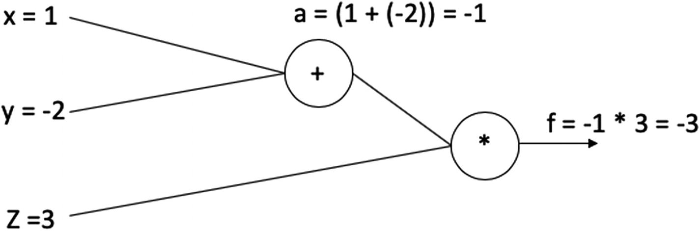
A computational graph with computed values
Now, with automatic differentiation, we would want to find the gradients of f with regard to the input variables (x, y, and z) represented as  ,
, and
and  .
.
In the feed-forward network, essentially, we find the gradients of the loss function with respect to the weights. To solve this, we can use the chain rule.
Let’s find the partial derivatives for the above equation.
We know that a = (x + y), z = a * x and thus f = az.
Therefore,
 = (x + y) = (1 – 2) = -1

If we go one step further, we can find the partial derivatives of a with regard to x and y.
 , and
, and 


We now have computed all the values required.
 = 3 and
  = -1
= -1
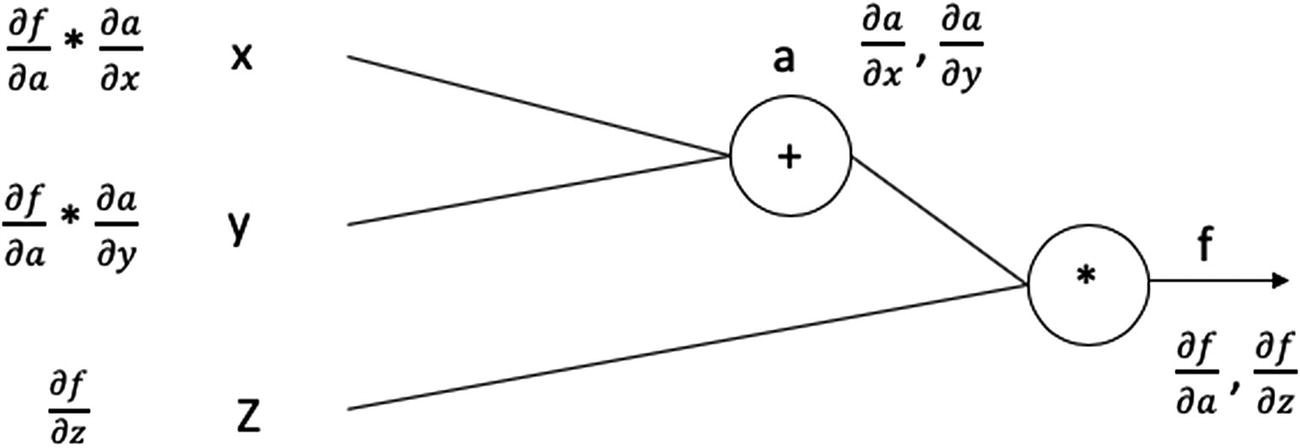
A computational graph with partial derivatives
Implementing Automatic Differentiation
Let’s now consider how automatic differentiation is implemented within PyTorch. The preceding example was very simple; things would be really complicated as we explore the approach on paper for large functions (i.e., deep learning functions). In most common networks, the number of parameters that would be involved is very high, making manually programming the computation of gradients a herculean task.
PyTorch provides the Autograd package, which essentially simplifies the entire process for us. Recall the loss.backward() function that we leveraged in Chapter 3 for the toy neural network. The network computes all the necessary gradients for the loss with respect to the weights. Let’s explore this further.
What Is Autograd?
The Autograd package within PyTorch provides automatic differentiation for all operations on tensors. It performs the necessary computations within backpropagation for our neural network. When the backward() function is called, the module computes all the backpropagation gradients automatically. We can also access individual gradients through a variable’s grad attribute.
The Autograd module provides ready to use tools (functions/classes) for implementing automatic differentiation of arbitrary scalar valued functions. To enable gradients to be computed for a variable, we need only to set the value as True for the keyword requires_grad.
Implementing Automatic Differentition (Autograd) in PyTorch
The gradient values here match exactly with what we computed manually earlier.
While we define a network in PyTorch, a lot of these details are taken care of. When we define a network layer, with nn.Linear(64, 256) (refer to the Chapter 3 example), PyTorch creates the weight and bias tensor with the necessary values (setting requires_grad as True). The input tensors did not need the gradients; hence, we never set them in our example and used the default (i.e., False).
Summary
This chapter covered the basics of automatic differentiation. Backpropagation is a special case of automatic differentiation used in training deep neural networks. In modern deep learning literature, automatic differentiation is analogous to backpropagation, as it a more generalized term. The key takeaway from this chapter is that automatic differentiation enables the computation of gradients for arbitrarily complex loss functions and is one of the key enabling technologies for deep learning. You should internalize the concepts of automatic differentiation and how it differs from both symbolic and numerical differentiation.
In the next chapter, we will study some additional topics related to deep learning in more detail, including performance metrics and model evaluation, analyzing overfitting and underfitting, regularization, and hyperparameter tuning. Finally, we will combine all the foundational bits about deep learning we’ve covered so far into a practical example that implements feed-forward neural networks for a real-world dataset.