This chapter covers

• Revisiting the dataset and determining which features to use to train the model
• Refactoring the dataset to include timeslots when there is no delay
• Transforming the dataset into the format expected by the Keras model
• Building a Keras model automatically based on the structure of the data
• Examining the structure of the model
• Setting parameters, including activation and optimization functions and learning rate

This chapter begins with a quick reexamination of the dataset to consider which columns can legitimately be used to train the model. Then we’ll go over the transformations required to get the data from the format in which we have been manipulating it (Pandas dataframes) to the format expected by the deep learning model. Next, we will go over the code for the model itself and see how the model is built up layer by layer based on the category of the input columns. We wrap up by reviewing methods you can use to examine the structure of the model and the parameters you can use to adjust how the model is trained.

All the preceding chapters in this book have been building up to this point. After examining the problem, preparing the data, we are finally ready to dig into the deep learning model itself. One thing to keep in mind as you go through this chapter: if you have not worked directly with deep learning models before, you may find the code for the model to be somewhat anticlimactic after all the detailed work required to prepare the data. This feeling may be familiar to you from using Python libraries for classic machine learning algorithms. The code to apply logistic regression or linear regression to a dataset that has been prepared for training isn’t exciting, particularly if you have had to create nontrivial code to tame a real-world dataset. You can see the code described in this chapter in the streetcar_ model_training notebook.

5.1 Data leakage and features that are fair game for training the model

Before we get into the details of the code that constitutes the model, we need to review which columns (either columns from the original dataset or columns derived from the original columns) are legitimate to use to train the model. If we need to use the model to predict streetcar delays, we need to ensure that we avoid data leakage. Data leakage occurs when you train a model using data (including the outcome that you’re trying to predict) from outside the training dataset. If you succumb to data leakage when you train a model by depending on data that isn’t available at the point when you want to make a prediction, you risk the following problems:

• Undermining your ability to make predictions

• Getting a performance measurement for your model that is too optimistic

To understand the problem of data leakage, consider a simple model that predicts the sale price of houses in a given property market. For this model, you have a set of information about houses that have sold recently in this market. You can use this information to train a model that you will later use to predict the sales price of houses that are being put on the market, as shown in figure 5.1.

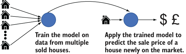
Figure 5.1 Training and applying a model to predict house prices

Figure 5.2 shows the features that are available for you to choose from in the sold-houses dataset.

Figure 5.2 Features available in the dataset of sold houses

Our goal is to make a prediction about the selling price for a house when it initially goes on the market, potentially weeks before it sells. When the house is ready to go on the market, the following features will be available:

• Number of bedrooms

• Number of bathrooms

• Floor space

• Frontage

We know that selling price (the feature that we want to predict) won’t be available. What about these features?

• Time on market

• Asking price

Time on market won’t be available when we want to make a prediction because the house has not been on the market yet, so we should not use this feature to train the model. Asking price is a bit more ambiguous; it may or may not be available at the point when we want to make the prediction. This example shows that we need a deeper understanding of the real-world business situation before we can determine whether a given feature will lead to data leakage.

5.2 Domain expertise and minimal scoring tests to prevent data leakage

What can you do to prevent the data leakage problems described in section 5.1? If you already have domain expertise in the business problem that your deep learning model is trying to solve, it will be easier for you to avoid data leakage. One of the rationales for this book is to enable you to exercise deep learning on problems in your everyday work so that you can take advantage of the domain expertise that you possess from doing your job.

Returning to the house-prices example (section 5.1), what would happen if you trained your model using features that have been identified as sources of data leakage, such as time on market? First, during the training, you probably would see model performance (measured by accuracy, for example) that looks good. This great performance, however, is misleading. It’s the equivalent of a teacher being happy about her students’ performance on a test when every student had a peek at the answers during the test. The students didn’t legitimately do well because they were exposed to information that should not have been available to them at the time of the test. The second result of data leakage is that when you finish training the model and try to apply it, you will find that some of the features that you need to feed the model to get a prediction are missing.

In addition to applying domain knowledge (such as the time on market not being known when a house first goes on the market), what can you do to prevent data leakage? A minimal scoring test on an early iteration of the model can help. In the house-prices example, we could take a provisional version of the trained model and apply data from one or two houses that are newly on the market. The prediction may be poor because the training iterations are not complete, but this exercise will expose features the model requires that aren’t available at prediction time, allowing us to remove them from the training process.

5.3 Preventing data leakage in the streetcar delay prediction problem

In the streetcar delay example, we want to predict whether a given streetcar trip is going to be delayed. In this context, including the Incident column as a feature to train the model would constitute data leakage, because before the trip is taken, we don’t know whether a given trip will have a delay and, if so, the nature of the delay. We don’t know what, if any, value the Incident column will have for a given streetcar trip before the trip is taken.

As shown in figure 5.3, the Min Delay and Min Gap columns also cause data leakage. Our label (the value we are trying to predict) is derived from Min Delay and is correlated with Min Gap, so both of these columns are potential sources of data leakage. We won’t know these values when we want to predict whether a given streetcar trip is going to be delayed.

Figure 5.3 Columns in the original dataset that can cause data leakage

Looking at the problem another way, which columns contain information that will be legitimately available to us when we want to make delay predictions for a particular trip or a set of trips? The information that the user provides at prediction time is described in chapter 8. The information provided by the user depends on the type of deployment:

• Web (figure 5.4)—In the web deployment of the model, the user selects seven scoring parameters (route, direction, and date/time details) that will be fed into the trained model to get a prediction.

  
  

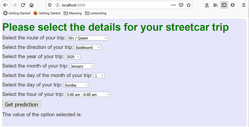
  Figure 5.4 Information provided by the user in the web deployment of the model

• Facebook Messenger (figure 5.5)—In the Facebook Messenger deployment of the model, the date/time details default to the current time when the prediction is made if the user doesn’t provide them explicitly. In this deployment, the user needs to provide only two scoring parameters: the route and the direction of their intended streetcar trip.

  
  

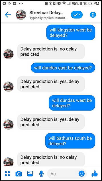
  Figure 5.5 Information provided by the user in the Facebook Messenger deployment of the model

Let’s check these parameters to ensure that we’re not risking data leakage:

• Route —When we want to predict whether a streetcar trip will be delayed, we’ll know what route (such as Route 501 Queen or Route 503 Kingston Road) the trip will take.

• Direction —We’ll know the direction (northbound, southbound, eastbound or westbound) of the trip at the time we want to predict whether it will be delayed.

We will also know the following date/time information (because the user sets the values explicitly in the web deployment or because we assume the current date/time in the Facebook Messenger deployment):

• Hour

• Day (day of the week, such as Monday)

• Day of month

• Month

• Year

We’d like to include one more feature in the data entry for predictions: Location. This feature is a bit trickier. If we look at the Location information in the source dataset as shown in figure 5.6, we know that we won’t have this information when we want to predict whether a streetcar trip will have delays. But we will know the start and end points of the trip (such as a trip on the 501 Queen route starting at Queen and Sherbourne and going to Queen and Spadina).

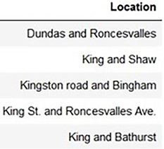
Figure 5.6 Values in the Location column

How can we correlate these start and end points with the likelihood that a delay will occur at a particular point on the trip? Unlike subway lines, which have stations that define distinct portions of the route, streetcar routes are fairly fluid. Many stops occur along a route, and these stops are not static, like those at subway stations; streetcar stops get moved. One approach that we will investigate in chapter 9 is dividing each route into sections and predicting whether a delay will occur in any of the sections that make up the entire trip along the streetcar route. For now, we are going to examine a version of the model that doesn’t include location data so that we can go through the model from end to end the first time without too much additional complexity.

If we limit ourselves to training the streetcar delay model to the columns we have identified (route, direction, and the date/time columns), we can prevent data leakage and be confident that the model we are training will be capable of making predictions about new streetcar trips.

5.4 Code for exploring Keras and building the model

When you have cloned the GitHub repo (http://mng.bz/v95x) associated with this book, you’ll find the code related to exploring Keras and building the streetcar delay prediction model in the notebooks subdirectory. The next listing shows the files that contain the code described in this chapter.

Listing 5.1 Code in the repo related to exploring Keras and building the model

├── data                                          ❶ 
│ 
├── notebooks
│ streetcar_model_training.ipynb        ❷ 
│           streetcar_model_training_config.yml   ❸ 
│ keras_sequential_api_mnist.py         ❹ 
│ keras_functional_api_mnist.py         ❺ 

❶ Directory for the pickled dataframe that is the output of the data preparation steps

❷ Notebook containing code to refactor the input dataset and build the model

❸ Config file for the model training notebook, with parameters including the name of the pickled dataframe that is input to the model training notebook

❹ Example of using the Keras sequential API to define a simple deep learning model (see section 5.10 for details)

❺ Example of using the Keras functional API to define a simple deep learning model (see section 5.10 for details)

5.5 Deriving the dataframe to use to train the model

In chapters 1-4, we went through many steps to clean and transform the data, including

• Replacing redundant values with a single consistent value, such as replacing eastbound , e/b , and eb with e in the Direction column

• Removing records with invalid values, such as records with Route values that aren’t valid streetcar routes

• Replacing categorical values with numeric identifiers

Figure 5.7 shows the outcomes of these transformations.

Figure 5.7 The input dataset after the transformations up to the end of chapter 4

Will this dataset be sufficient to train a model to meet our goal of predicting whether a given streetcar trip will be delayed? The answer is no. As it stands now, this dataset has only records for delays. What’s missing is information about all the situations when there were no delays. What we need is a refactored dataset that also has records of all the times when there were no delays on a particular route in a particular direction.

Figure 5.8 summarizes the difference between the original dataset and the refactored dataset. In the original dataset, every record describes a delay, including the time, route, direction, and incident that caused the delay. In the refactored dataset, there is a record for every combination of time slot (every hour since January 1, 2014), route, and direction, whether or not there was a delay on that route in that direction during that time slot.

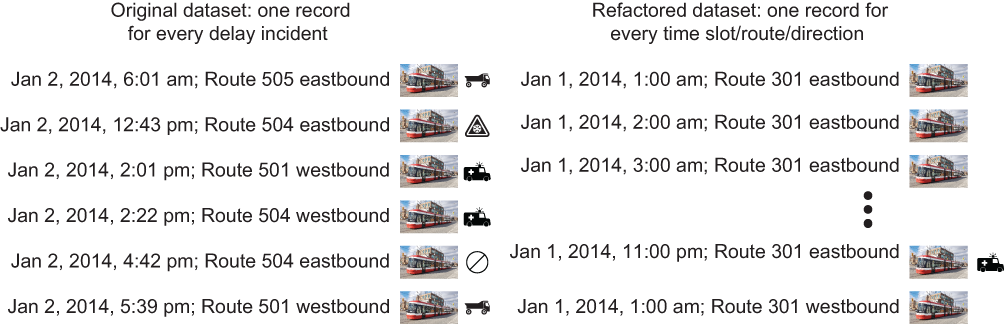
Figure 5.8 Comparing the original dataset with the refactored dataset

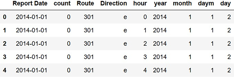
Figure 5.9 shows explicitly what the refactored dataset looks like. If there is a delay in a given time slot (an hour in a particular day) on a given route in a given direction, count is nonzero; otherwise, count is zero. The snippet of the refactored dataset in figure 5.9 shows that there were no delays on Route 301 in the eastbound direction between midnight and 5 a.m. on January 1, 2014.

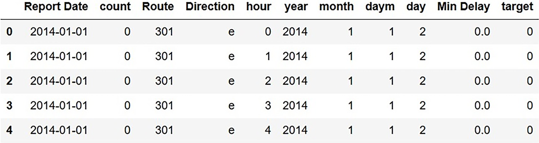
Figure 5.9 Refactored dataset with a row for each route/direction/time-slot combination

Figure 5.10 summarizes the steps to get the refactored dataset that has an entry for every time-slot/route/direction combination.

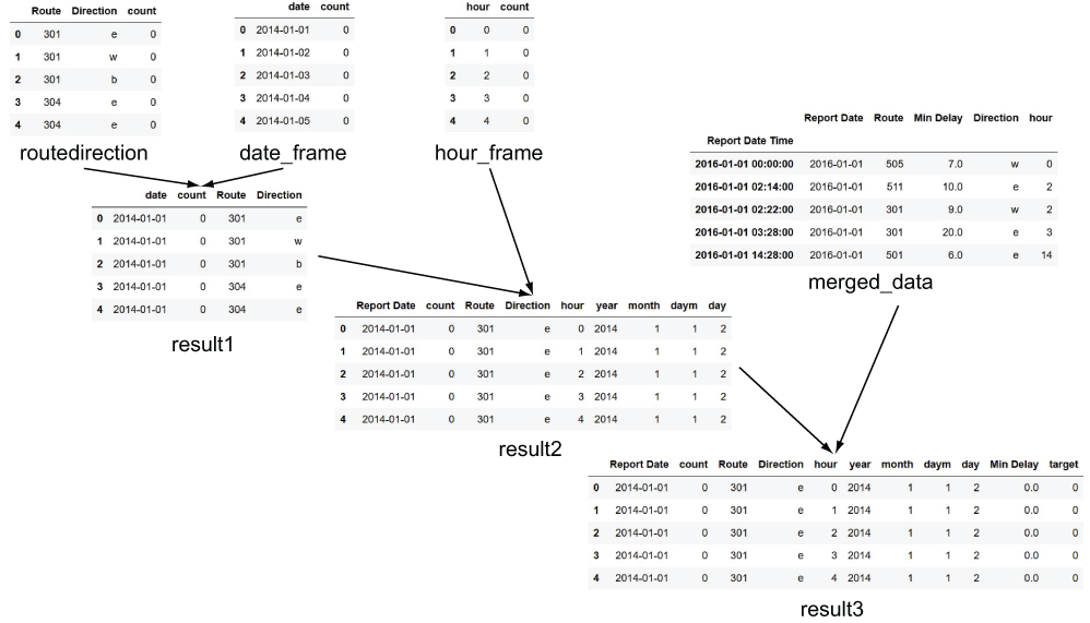
Figure 5.10 Refactoring the dataframe

Following are the steps:

1. Create a routedirection_frame dataframe containing a row for each route/ direction combination (figure 5.11).

Figure 5.11 routedirection_frame dataframe

1. Create a date_frame dataframe, containing a row for each date in the period from which training data will be selected (figure 5.12).

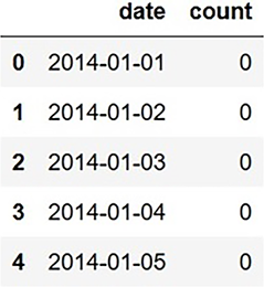
Figure 5.12 date_frame dataframe

1. Create an hour_frame dataframe, containing a row for each hour of the day (figure 5.13).

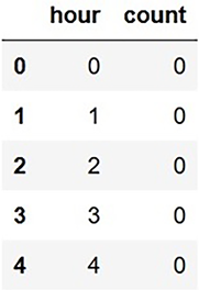
Figure 5.13 hour_frame dataframe

1. Combine these three dataframes to get the result2 dataframe (figure 5.14).

Figure 5.14 result2 dataframe

1. Add derived columns for the components of the date to the result2 dataframe:

   result2['year'] = pd.DatetimeIndex(result2['Report Date']).year
       result2['month'] = pd.DatetimeIndex(result2['Report Date']).month
       result2['daym'] = pd.DatetimeIndex(result2['Report Date']).day
       result2['day'] = pd.DatetimeIndex(result2['Report Date']).weekday 

2. Drop extraneous columns from the input dataset (merged_data dataframe) and combine it with the result2 dataframe to get the completed refactored dataframe (figure 5.15).

   
   

   Figure 5.15 Completed refactored dataframe

To compare the size of the dataset before and after refactoring, a dataset with 56,000 rows results in a refactored dataset with 2.5 million rows to cover a five-year period. The start and end of the time period covered by this refactored dataset is controlled by these variables, defined in the overall parameters block:

start_date =  date(config['general']['start_year'], 
config['general']['start_month'], config['general']['start_day'])
end_date = date(config['general']['end_year'], 
config['general']['end_month'], config['general']['end_day'])

The start date corresponds with the beginning of the delay dataset in January 2014. You can change the end date by updating the parameters in the config file streetcar_ model_training_config.yml, but note that you want to keep end_date no later than the latest delay data from the original source (http://mng.bz/4B2B).

5.6 Transforming the dataframe into the format expected by the Keras model

The Keras model expects tensors as input. You can think of a tensor as being a generalization of a matrix. A matrix is a 2D tensor, and a vector is a 1D tensor. Figure 5.16 summarizes common terms for tensors by dimension.

Figure 5.16 Tensor summary

When we have made all the data transformations that we need to make in Pandas dataframes, the final step before feeding this data into the model to train is putting the data in the tensor format required by the Keras model. By leaving this transformation as the final step before training the model, we get to enjoy the convenience and familiarity of Pandas dataframes until we need to put the data in the format expected by the Keras model. The code to perform this transformation is in the transform method of the prep_for_keras_input class, shown in the next listing. This class is part of the pipelines described in chapter 8 that perform transformations on data for training and scoring.

Listing 5.2 Code to put the data in the tensor format required by the model

def __init__(self):
        self.dictlist = []                               ❶ 
        return None
 
 
def transform(self, X, y=None, **tranform_params):
        for col in self.collist:
            print("cat col is",col)
            self.dictlist.append(np.array(X[col]))       ❷ 
        for col in self.textcols:
            print("text col is",col)
            self.dictlist.append(pad_sequences(X[col], 
            ➥ maxlen=max_dict[col]))                    ❸ 
        for col in self.continuouscols:
            print("cont col is",col)
            self.dictlist.append(np.array(X[col]))       ❹ 
        return self.dictlis.t

❶ List that will contain numpy arrays for each column

❷ Append the numpy array for the current categorical column to the overall list.

❸ Append the numpy array for the current text column to the overall list.

❹ Append the numpy array for the current continuous column to the overall list.

This code is flexible. Like the rest of the code in this example, as long as the columns from the input dataset are categorized correctly, this code will work with a wide variety of tabular structured data. It isn’t specific to the streetcar dataset.

5.7 A brief history of Keras and TensorFlow

We have reviewed the final set of transformations that the dataset needs to go through in preparation to train a deep learning model. This section provides background on Keras, the high-level deep learning framework used to create the model for the primary example in this book. We will begin in this section by briefly reviewing the history of Keras and its relationship with TensorFlow, the low-level deep learning framework. In section 5.8, we will review the steps required to migrate from TensorFlow 1.x to TensorFlow 2, the backend deep learning framework used for the code examples in this book. In section 5.9, we will briefly contrast the Keras/TensorFlow framework with the other major deep learning framework, PyTorch. In section 5.10, we will review two code examples that show how the layers of a deep learning model are built in Keras. With this background on Keras, we will be ready to examine how the Keras framework is used to implement the streetcar delay prediction deep learning model in section 5.11.

Keras began its life as a frontend for a variety of backend deep learning frameworks, including TensorFlow (https://www.tensorflow.org) and Theano. The purpose of Keras was to provide a set of accessible, easy-to-use APIs that developers could use to explore deep learning. When Keras was released in 2015, the deep learning backend libraries that it supported (first Theano and then TensorFlow) provided a broad range of functions but could be challenging for beginners to master. With Keras, developers could get started with deep learning by using familiar syntax and without having to worry about all the details exposed in the backend libraries.

If you were starting a deep learning project back in 2017, your choices included

• Using TensorFlow libraries directly

• Using Keras as a frontend to TensorFlow

• Using Keras with another backend, such as Theano (although by 2017 backends other than TensorFlow were becoming rare)

Although most people who used Keras for deep learning projects exploited TensorFlow as the backend, Keras and TensorFlow were distinct, separate projects. All this changed in 2019 with the release of TensorFlow 2:

• Coders using Keras for deep learning are encouraged to use the tf.keras package integrated into TensorFlow rather than free-standing Keras.

• TensorFlow users are encouraged to use Keras (via the tf.keras package in TensorFlow) as the high-level API for TensorFlow. As of TensorFlow 2, Keras is the official high-level API for TensorFlow (http://mng.bz/xrWY).

In short, Keras and TensorFlow, which had originally been separate but related projects, have come together. In particular, as new TensorFlow point releases come out (such as TensorFlow 2.2.0 [http://mng.bz/yrnJ ], released in May 2020), they will include improvements in the backend as well as improvements in the Keras frontend. You can find more details about the relationship between Keras and TensorFlow, particularly the role played by TensorFlow in the overall operation of a deep learning model defined with Keras, in the Deep Learning with Python chapter on Keras and TensorFlow (http://mng.bz/AzA7).

5.8 Migrating from TensorFlow 1.x to TensorFlow 2

The deep learning model code described in this chapter and chapter 6 was originally written to use self-standing Keras with TensorFlow 1.x as a backend. TensorFlow 2 was released while this book was being written, so I decided to migrate to the integrated Keras environment in TensorFlow 2. Thus, to run the code in streetcar_model_training .ipynb , you need to have TensorFlow 2 installed in your Python environment. If you have other deep learning projects that have not moved to TensorFlow 2, you can create a Python virtual environment specifically for the code example in this book and install TensorFlow 2 there. That way, you will not introduce changes in your other deep learning projects.

This section summarizes the changes that I needed to make to the code in the model training notebook to migrate it from self-standing Keras with TensorFlow 1.x as a backend to Keras in the context of TensorFlow 2. The TensorFlow documentation includes comprehensive migration steps at https://www.tensorflow.org/guide/migrate. Following is a brief summary of the steps I took:

1. Upgraded my existing level of TensorFlow to the latest TensorFlow 1.x level:

   pip install tensorflow==1.1.5

2. Ran the model training notebook end to end to validate that everything worked in the latest level of TensorFlow 1.x.

3. Ran the upgrade script tf_upgrade_v2 on the model training notebook.

4. Changed all Keras import statements to reference the tf.keras package (including changing from keras import regularizers to from tensorflow.keras import regularizers).

5. Ran the model training notebook end to end with the updated import statements to validate that everything worked.

6. Created a Python virtual environment, following the instructions at https:// janakiev.com/blog/jupyter-virtual-envs.

7. Installed TensorFlow 2 in the Python virtual environment. This step was necessary because the Rasa chatbot framework that is part of the Facebook Messenger deployment approach described in chapter 8 requires TensorFlow 1.x. By installing TensorFlow 2 in a virtual environment, we can exploit the virtual environment for the model training steps without breaking the deployment prerequisite for TensorFlow 1.x. Here is the command to install TensorFlow 2:

   pip install tensorflow==2.0.0

The process of migrating to TensorFlow 2 was painless, and thanks to Python virtual environments, I was able to apply this migration where I needed it for the model training without causing any side effects for the rest of my Python projects.

5.9 TensorFlow vs. PyTorch

Before exploring Keras in more depth, it’s worth quickly discussing the other major library that is currently used for deep learning: PyTorch (https://pytorch.org). PyTorch was developed by Facebook and made available as open source in 2017. The article at http://mng.bz/Moj2 makes a succinct comparison of the two libraries. The community that uses TensorFlow is currently larger than the one that uses PyTorch, although PyTorch is growing quickly. PyTorch has a stronger presence in the academic/research world (and is the basis of the coding aspects of the fast.ai course described in chapter 9), whereas TensorFlow is predominant in industry.

5.10 The structure of a deep learning model in Keras

You may recall that chapter 1 described a neural network as a series of nodes organized in layers, each of which has weights associated with it. In simple terms, during the training process these weights get updated repeatedly until the loss function is minimized and the accuracy of the model’s predictions is optimized. In this section, we will show how the abstract idea of layers introduced in chapter 1 is manifested in code in Keras by reviewing two simple deep learning models.

There are two ways to define the layers of a Keras model: the sequential API and the functional API. The sequential API is the simpler method but is less flexible; the functional API has more flexibility but is a bit more complex to use.

To illustrate these two APIs, we are going to look at how we would create minimal Keras deep learning models with both approaches for MNIST (https://www.tensorflow .org/datasets/catalog/mnist). If you have not encountered MNIST before, it is a dataset made up of labeled images of handwritten digits. The x values come from the image files, and the labels (y values) are the text representations of the digits. The goal of a model exercising MNIST is to correctly identify the digit for the handwritten images. MNIST is commonly used as a minimal dataset for exercising deep learning models. If you want more background on MNIST and how it is used to exercise deep learning frameworks, a great article at http://mng.bz/Zr2a provides more details.

It is worth noting that MNIST is not a structured dataset according to the definition of structured data in chapter 1. There are two reasons for choosing MNIST for the examples in this section, even though it’s not a structured dataset: the published starter examples of the Keras APIs use MNIST, and there is no recognized structured dataset for exercising deep learning models that is equivalent to MNIST.

With the sequential API, the model definition takes as an argument an ordered list of layers. You can select layers that you want to include in your model from the list of supported Keras layers in TensorFlow 2 (http://mng.bz/awaJ). The code snippet in listing 5.3 comes from keras_sequential _api_mnist.py. It is adapted from the TensorFlow 2 documentation (http://mng.bz/ RMAO) and shows a simple deep learning model for MNIST that uses the Keras sequential API.

Listing 5.3 Code for an MNIST model using the Keras sequential API

import tensorflow as tf
import pydotplus
from tensorflow.keras.utils import plot_model
 
mnist = tf.keras.datasets.mnist 
 
(x_train, y_train), (x_test, y_test) = mnist.load_data()
x_train, x_test = x_train / 255.0, x_test / 255.0
 
model = tf.keras.models.Sequential([                         ❶ 
  tf.keras.layers.Flatten(input_shape=(28, 28)),             ❷ 
  tf.keras.layers.Dense(128, activation='relu'),             ❸ 
  tf.keras.layers.Dropout(0.2),                              ❹ 
  tf.keras.layers.Dense(10)                                  ❺ 
])
 
model.compile(optimizer='adam',
              loss=tf.keras.losses.SparseCategoricalCrossentropy(from_logits=True),
              metrics=['accuracy'])                          ❻ 
 
history = model.fit(x_train, y_train, 
                    batch_size=64, 
                    epochs=5, 
                    validation_split=0.2)                    ❼ 
 
                   
test_scores = model.evaluate(x_test,  y_test, verbose=2)     ❽ 
print('Test loss:', test_scores[0])
print('Test accuracy:', test_scores[1])

❶ Define Keras sequential model

❷ Flatten layer that reshapes the input tensor to a tensor with a shape equal to the number of elements in the input tensor

❸ Dense layer that does the standard operation of getting the dot product of the input to the layer and the weights in the layer, plus the bias

❹ Dropout layer that randomly turns off a proportion of the network

❺ Output dense layer

❻ Compile the model, specifying the loss function, the optimizer, and the metric to be tracked in the training process.

❼ Fit the model by adjusting the weights to minimize the loss function.

❽ Assess model performance

This simple example of a Keras deep learning model has several characteristics in common with non-deep-learning models that you have already seen:

• The input dataset is split into train and test subsets. The train subset is used in the training process to adjust the weights in the model. The test dataset is applied to the trained model to assess its performance; in this example, according to the accuracy (that is, how closely the predictions for the model match the actual output values).

• Both the training and test datasets are made up of input x values (for MNIST, images of handwritten digits) and labels or y values (for MNIST, the ASCII digits corresponding to the handwritten digits).

• Both non-deep-learning and deep learning models have similar statements to define and fit the model. The code snippets in the next listing contrast the statements to define and fit a logistic regression model and a Keras deep learning model.

• Listing 5.4 Code to contrast a logistic regression model and a Keras model

  from sklearn.linear_model import LogisticRegression
   
  clf_lr = LogisticRegression(solver = 'lbfgs')         ❶ 
  model = clf_lr.fit(X_train, y_train)                  ❷ 
   
  model = tf.keras.models.Sequential([                  ❸ 
    tf.keras.layers.Flatten(input_shape=(28, 28)),
    tf.keras.layers.Dense(128, activation='relu'), 
    tf.keras.layers.Dropout(0.2), 
    tf.keras.layers.Dense(10) 
  ])
  model.compile(optimizer='adam',                      ❹ loss=tf.keras.losses.SparseCategoricalCrossentropy(from_logits=True),
                metrics=['accuracy']) 
   
  history = model.fit(x_train, y_train,                ❺ 
                      batch_size=64, 
                      epochs=5, 
                      validation_split=0.2)

  ❶ Define the logistic regression model.

  ❷ Fit the logistic regression model.

  ❸ First part of defining the Keras deep learning model: defining the layers

  ❹ Second part of defining the Keras deep learning model: setting the compilation parameters

  ❺ Fit the Keras deep learning model.

Figure 5.17 shows the output of the plot_model function for the MNIST sequential API model.

Figure 5.17 plot_model output for simple sequential API Keras model

By contrast with the sequential API, the Keras functional API has a more complex syntax but provides greater flexibility. In particular, the functional API allows you to define a model with multiple inputs. As you will see in section 5.13, the extended example in this book exploits the functional API because it requires multiple inputs.

The code snippet in listing 5.5 comes from keras_ functional_api_mnist.py. It is adapted from https://www .tensorflow.org/guide/keras/functional and shows how you would use the Keras functional API to define a simple deep learning model for the same MNIST problem for which we showed a sequential API solution.

Listing 5.5 Code for an MNIST model using the Keras functional API

import numpy as np
import tensorflow as tf
from tensorflow import keras
from tensorflow.keras import layers
 
inputs = keras.Input(shape=(784,)) 
flatten = layers.Flatten(input_shape=(28, 28))                    ❶ 
flattened = flatten(inputs)
dense = layers.Dense(128, activation='relu')(flattened)           ❷ 
dropout = layers.Dropout(0.2) (dense)                             ❸ 
outputs = layers.Dense(10) (dropout)                              ❹ 
 
# define model inputs and outputs (taken from layer definition)
 
model = keras.Model(inputs=inputs, outputs=outputs, 
name='mnist_model')
(x_train, y_train), (x_test, y_test) = keras.datasets.mnist.load_data()
 
x_train = x_train.reshape(60000, 784).astype('float32') / 255 
x_test = x_test.reshape(10000, 784).astype('float32') / 255
 
# compile model, including specifying the loss function, 
optimizer, and metrics
 
model.compile(loss=keras.losses.SparseCategoricalCrossentropy( 
from_logits=True), 
     optimizer=keras.optimizers.RMSprop(), 
     metrics=['accuracy'])                                        ❺ 
 
# train model
 
history = model.fit(x_train, y_train, 
                    batch_size=64, 
                    epochs=5, 
                    validation_split=0.2)                         ❻ 
 
# assess model performance
 
test_scores = model.evaluate(x_test, y_test, verbose=2)           ❼ 
print('Test loss:', test_scores[0])
print('Test accuracy:', test_scores[1])

❶ Define layer that flattens the input tensor by reshaping it to a tensor with a shape equal to the number of elements in the input tensor

❷ Dense layer that does the standard operation of getting the dot product of the input to the layer and the weights in the layer, plus the bias

❸ Dropout layer that randomly turns off a proportion of the network

❹ Output dense layer

❺ Compile the model, specifying the loss function, the optimizer, and the metric to be tracked in the training process.

❻ Fit the model (with parameters set for the training dataset, batch size, number of epochs, and subset of the training set to reserve for validation) by adjusting the weights to minimize the loss function.

❼ Assess the model performance.

You can see a lot of similarity between the sequential API and functional API approaches to this problem. The loss function is defined the same way, for example, and the compile and fit statements are the same. What is different between the sequential API and the functional API is the definition of the layers. In the sequential API approach, the layers are defined in a single list, whereas in the functional API approach, the layers are recursively defined, with each layer being built on its predecessors.

Figure 5.18 shows the output of plot_model for this simple functional API Keras model.

Figure 5.18 plot_model output for the simple functional API Keras model

In this section, we have examined a couple of simple Keras models and reviewed the essential characteristics of two approaches offered in Keras: the sequential API and the functional API. In section 5.13, we will see how the streetcar delay prediction model takes advantage of the flexibility of the functional API.

5.11 How the data structure defines the Keras model

In chapter 3, you learned that the columns in the structured dataset are categorized as categorical, continuous, or text (figure 5.19).

Figure 5.19 Column categories in the streetcar dataset

• Continuous — These values are numeric. Examples of common continuous values include temperatures, currency values, time spans (such as elapsed hours), and counts of objects or activities. In the streetcar example, Min Delay and Min Gap (the columns containing the number of minutes of delay incurred by the delay and the length in minutes of the resulting gap between streetcars) are continuous columns. The latitude and longitude values derived from the Location column are also treated as continuous columns.

• Categorical —These values can be single strings, such as the days of the week, or collections of one or more strings that constitute an identifier, such as the names of the U.S. states. The number of distinct values in categorical columns can range from two to several thousand. Most of the columns in the streetcar dataset are categorical, including Route, Day, Location, Incident, Direction, and Vehicle.

• Text —These values are sets of strings.

It’s essential to organize the input dataset into these categories because the categories define how the deep learning model code is assembled in the deep learning approach described in this book. The layers of the Keras model are built up based on these categories, with each category having its own structure of layers.

The following illustrations summarize the layers that are built up for categorical and text columns. Figure 5.20 shows the layers that get built for categorical columns:

• Embedding —As explained in section 5.12, embeddings provide a way for the model to learn the relationships between values in categorical categories in the context of the overall prediction the model is making.

• Batch normalization —Batch normalization is a method of preventing overfitting (a model working well on the dataset it was trained on, but poorly on other data) by controlling how much weights change in hidden layers.

• Flatten —Reshape the input to prepare for subsequent layers.

• Dropout —Use this technique to prevent overfitting. With dropout, as the name suggests, rotating, random subsets of nodes in the network are ignored in forward and backward passes through the network.

• Concatenate —Join the layers for this input with layers for the other inputs.

  
  

  Figure 5.20 Keras layers for categorical inputs

Figure 5.21 shows the layers that get built for text input columns. In addition to the layers for categorical columns, text columns get a GRU layer. A GRU (https://keras .io/api/layers/recurrent_layers/gru) is a kind of recurrent neural network (RNN), the class of deep learning models commonly used for text processing. What sets RNNs apart from other neural networks are the gates that control how much previous inputs affect the way that current input changes weights in the model. The interesting point is that the actions of these gates—how much is “remembered” from previous input—is learned in the same way that the generic weights in the network are learned. Adding this layer to the set of layers for text columns means, at a high level, that the order of words in the text column (not the presence of individual words alone) contributes to the training of the model.

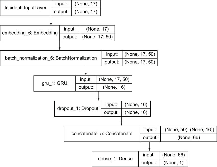
Figure 5.21 Keras layers for text inputs

We’ve reviewed the layers that are added to the deep learning model for categorical and text columns. What about continuous columns? These columns don’t have any special additional layers and are concatenated directly into the overall model.

This section briefly described the layers in the deep learning model that are built up for each of the three column types in a structured dataset: continuous, categorical, and text. In section 5.13, we will go in detail through the code that implements these layers.

5.12 The power of embeddings

In section 5.11, you saw the layers that get defined for each type of column in a structured dataset. In particular, you saw that categorical and text columns get embedding layers. In this section, we will examine embeddings and how they are used. We will return to the power of embeddings in chapter 7 in an experiment that demonstrates the effect of categorical column embeddings on the performance of the model.

Embeddings come from the world of natural language processing, in which they are used to map words to a numeric representation. Embeddings are an important topic for this book because they are essential for enabling a deep learning model to exploit categorical and text columns in a structured dataset. This section is not an exhaustive description of embeddings—a topic that deserves a book of its own—but it introduces the concept and describes why embeddings are needed in a deep learning project on structured data. You can find a more detailed description of embeddings in the section on text embeddings in Stephan Raaijmakers’s Deep Learning for Natural Language Processing (http://mng.bz/2WXm).

The excellent article at http://mng.bz/1gzn states that embeddings are representations of categorical values as learned, low-dimensional continuous vectors . That’s a lot of information in one sentence. Let’s look at it piece by piece:

• Representations of categorical values —Recall the definition of categorical values from chapter 3: These values can be “single strings, such as the days of the week, or collections of one or more strings that constitute an identifier, such as the names of the U.S. states. The number of distinct values in categorical columns can range from two to several thousand.” The columns in the streetcar dataset that have embeddings associated with them include the categorical columns Route, Day, Location, Incident, Direction, and Vehicle.

• Learned —Like the deep learning model weights introduced in chapter 1, the values of embeddings are learned. The values of embeddings are initialized before training and then get updated through iterations of the deep learning model. The result is that after the embeddings have been learned, the embeddings for categorical values that tend to produce the same outcome are closer to one another. Consider the context of days of the week (Monday to Sunday) as a derived feature of the streetcar delay dataset. Suppose that delays are less common on weekends. If this is the case, the embeddings learned for Saturday and Sunday will be closer to one another than to the embeddings learned for the weekdays.

• Low-dimensional —This term means that the dimension of the embedding vectors is low compared with the number of categorical values. In the model created for the main example in this book, the Route column has more than 1,000 distinct values but has an embedding with a dimension of 10.

• Continuous —This term means that the values in the embedding are represented by floating-point values as opposed to the integers that represent the categorical values themselves.

A famous illustration of embeddings (https://arxiv.org/pdf/1711.09160.pdf) demonstrates how they can capture the relationships between the categorical values with which they are associated. This illustration shows the relationship between the vectors associated with four words in Word2Vec (http://mng.bz/ggGR):

v(king) − v(man) + v(woman) ≈ v(queen)

This says that the embedding vector for king minus the embedding vector for man plus the embedding vector for woman is close to the embedding vector for queen. In this example, arithmetic on the embeddings matches the semantic relationship between the words associated with the embeddings. This example shows the power of embeddings to map non-numeric, categorical values to a planar space where the values can be manipulated like numbers.

A secondary benefit of embeddings is that they can be used to illustrate implicit relationships among categorical values. You get unsupervised learning analysis of the categories for free as you are solving the supervised learning problem.

A final benefit of embeddings is that they give you a way to incorporate categorical values into a deep learning framework without the drawbacks of one-hot encoding (http://mng.bz/P1Av). In one-hot encoding, if there are seven values (such as for the days of the week), each value is represented by a vector of size 7 with six 0 s and a single 1 :

• Monday: [1,0,0,0,0,0,0]

• Tuesday: [0,1,0,0,0,0,0,0]

• . . .

• Sunday: [0,0,0,0,0,0,0,1]

In a structured dataset, a one-hot encoding of the days-of-the-week category would require seven columns, which is not too bad for a category with a small number of values. But what about the Vehicle column, which has hundreds of values? You can see how one-hot encoding will quickly explode the number of columns in the dataset and the memory requirements to process the data. By exploiting embeddings in deep learning, we can deal with categorical columns without the poor scaling behavior of one-hot encoding.

This section is a brief introduction to the topic of embeddings. The benefits of using embeddings include the ability to manipulate non-numeric values that are analogous to common numeric operations, the ability to get unsupervised learning-type categorization on values in a categorical range as a byproduct of solving a supervised learning problem, and the ability to train deep learning models with categorical inputs without the drawbacks of one-hot encoding.

5.13 Code to build a Keras model automatically based on the data structure

The Keras model is made of up of a sequence of layers through which input columns flow to generate a prediction of a delay in a given route/direction/time-slot combination. Figure 5.22 shows the layers that the input columns flow through, depending on their data category (continuous, categorical, or text), along with examples of the kinds of data in each category. To examine the options you have for exploring these layers, see section 5.14.

Figure 5.22 Keras layers by column type with examples

The next listing shows the code that assigns each of the columns to one of these categories.

Listing 5.6 Code that assigns columns to categories

textcols = []                                               ❶ 
continuouscols = []                                         ❷ 
if targetcontinuous:
    excludefromcolist = ['count','Report Date', 'target', 
    ➥ 'count_md','Min Delay']                              ❸ 
else:
    excludefromcolist = ['count','Report Date', 
    ➥ 'target','count_md', 'Min Delay'] 
nontextcols = list(set(allcols) - set(textcols))
collist = list(set(nontextcols) - 
set(excludefromcolist) - set(continuouscols))               ❹ 

❶ The set of text columns in the refactored model is empty.

❷ The set of continuous columns in the refactored model is empty.

❸ excludefromcolist is the set of columns that will not train the model.

❹ collist is the list of categorical columns. Here, it is generated by taking the list of columns and removing the text columns, continuous columns, and excluded columns.

These column lists—textcols , continuouscols , and collist —are used throughout the code to determine what actions are taken on the columns, including how the layers of the deep learning model are built up for each column that is being used to train the model. The following sections show the layers added for each column type.

The following listing shows what the training data looks like before it is applied to the model for training. The training data is a list of numpy arrays—one array for each column in the training data.

Listing 5.7 Format of the data before being used to train the model

X_train_list is  
[array([13, 23,  2, ...,  9, 22, 16]),     ❶ 
array([13, 13,  3, ...,  4, 11,  2]),      ❷ 
array([1, 6, 5, ..., 5, 3, 2]),            ❸ 
array([8, 9, 0, ..., 7, 0, 4]),            ❹ 
array([4, 1, 1, ..., 1, 4, 4]),            ❺ 
array([10, 10, 23, ..., 21, 17, 15]),      ❻ 
array([4, 1, 3, ..., 0, 3, 0])]            ❼ 

❶ numpy array for hour. Values range from 0-23.

❷ numpy array for route. Values range from 0-14.

❸ numpy array for day of the week. Values range from 0-6.

❹ numpy array for month. Values range from 0-11.

❺ numpy array for year. Values range from 0-6.

❻ numpy array for day of the month. Values range from 0-30.

❼ numpy array for direction. Values range from 0 4.

The code that assembles the layers for each type of column is in the streetcar_ model_training notebook in the get_model() function. Following is the code block in get_model() for continuous columns, which simply have the input layer flow through:

for col in continuouscols: 
        continputs[col] = Input(shape=[1],name=col)
        inputlayerlist.append(continputs[col])

In the code block in get_model() for categorical columns, we see that these columns get embeddings and batch normalization layers, as the next listing shows.

Listing 5.8 Code to apply embeddings and batch normalization to categorical columns

for col in collist:
        catinputs[col] = Input(shape=[1],name=col)                   ❶ 
        inputlayerlist.append(catinputs[col])                        ❷ 
        embeddings[col] = 
        ➥ (Embedding(max_dict[col],catemb) (catinputs[col]))        ❸ 
        embeddings[col] = (BatchNormalization() (embeddings[col]))   ❹ 

❶ Start with the input.

❷ Append the input layer for this column to the list of input layers, which will be used in the model definition statement.

❸ Add the embedding layer.

❹ Add the batch normalization layer.

In the code block in get_model () for text columns, we see that these columns get layers for embeddings, batch normalization, dropout, and a GRU, as shown next.

Listing 5.9 Code to apply the appropriate layers to text columns

for col in textcols:
textinputs[col] = 
Input(shape=[X_train[col].shape[1]], name=col)                         ❶ 
inputlayerlist.append(textinputs[col])                                 ❷ 
textembeddings[col] = (Embedding(textmax,textemb) (textinputs[col]))   ❸ 
textembeddings[col] = (BatchNormalization() (textembeddings[col]))     ❹ 
textembeddings[col] = 
Dropout(dropout_rate)( GRU(16,kernel_regularizer=l2(l2_lambda)) 
(textembeddings[col]))                                                 ❺ 

❶ Start with the input.

❷ Append the input layer for this column to the list of input layers, which will be used in the model definition statement.

❸ Add the embedding layer.

❹ Add the batch normalization layer. By default, samples are normalized individually.

❺ Add the dropout layer and the GRU layer.

In this section, we’ve gone through the code that makes up the heart of the Keras deep learning model for the streetcar delay prediction problem. We’ve seen how the get_model() function builds up the layers of the model based on the types (continuous, categorical, and text) of the input columns. Because the get_model() function does not depend on the tabular structure of any particular input dataset, this function works with a wide variety of input datasets. Like the rest of the code in this example, as long as the columns from the input data set are categorized correctly, the code in the get_model() function will generate a Keras model for a wide variety of tabular structured data.

5.14 Exploring your model

The model that we have created to predict streetcar delays is relatively simple but can still be somewhat overwhelming to understand if you have not encountered Keras before. Luckily, you have utilities you can use to examine the model. In this section, we will review three utilities that you can use to explore your model: model.summary (), plot_model , and TensorBoard.

The model.summary() API lists each of the layers in the model, its output shape, the number of parameters, and the layer that is fed into it. The snippet of model .summary() output in figure 5.23 shows the input layers daym, year, Route, and hour. You can see how daym is connected to embedding_1, which is in turn connected to batch_normalization_1, which is connected to flatten_1.

Figure 5.23 model.summary() output

When you initially create a Keras model, the output of model.summary () can really help you understand how the layers are connected and validate your assumptions about how the layers are related.

If you want a graphical perspective of how the layers of the Keras model are related, you can use the plot_model function (https://keras.io/visualization). model.summary() produces information about the model in tabular format; the file generated by plot_ model illustrates the same information graphically. model.summary() is easier to use. Because plot_model is dependent on the Graphviz package (a Python implementation of the Graphviz [https://www.graphviz.org ] visualization software), it can take some work to get plot_model working in a new environment, but the effort pays off if you need an accessible way to explain your model to a wider audience.

Here is what I needed to do to get plot_model to work in my Windows 10 environment:

pip install pydot
pip install pydotplus
conda install python-graphviz

When I completed these Python library updates, I downloaded and installed the Graphviz package (https://graphviz.gitlab.io/download) in Windows. Finally, to get plot_model to work in Windows, I had to update the PATH environment variable to explicitly include the bin directory in the install path for Graphviz.

The following listing shows the code in the streetcar_model_training notebook that invokes plot_model.

Listing 5.10 Code to invoke plot_model

if save_model_plot:                                              ❶ 
    model_plot_file = "model_plot"+modifier+".png"               ❷ 
    model_plot_path = os.path.join(get_path(),model_plot_file)
    print("model plot path: ",model_plot_path)
    plot_model(model, to_file=model_plot_path)                   ❸ 

❶ Check whether the save_model_plot switch is set in the streetcar model training config file.

❷ If so, set the filename and path where the model plot will be saved.

❸ Call plot_model with the model object and the fully qualified filename as parameters.

Figure 5.24 and 5.25 show the output of plot_model for the streetcar delay prediction model. The start of the layers for each column is highlighted with a number:

1. Direction

2. Hour

3. Year

4. Route

5. Month

6. Day of month

7. Day

 

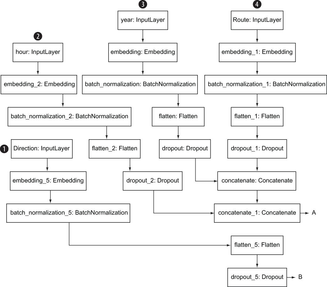
Figure 5.24 Output of plot_model showing the layers in the model (top portion)

Figure 5.25 Output of plot_model showing the layers in the model (bottom portion)

Figure 5.26 shows a closeup of plot_model output for the day column.

In addition to model .summary() and plot_model, you can use the TensorBoard utility to examine the characteristics of a trained model. TensorBoard (https://www. tensorflow.org/tensorboard/get_started) is a tool provided with TensorFlow that allows you to graphically track metrics such as loss and accuracy, and to generate a diagram of the model graph.

Figure 5.26 Closeup of the layers for the day column

To use TensorBoard with the streetcar delay prediction model, follow these steps:

1. Import the required libraries:

   from tensorflow.python.keras.callbacks import TensorBoard

2. Define a callback for TensorBoard that includes the path for TensorBoard logs, as shown in this snippet from the set_early_stop function in the streetcar_ model_training notebook.

   Listing 5.11 Code to define callbacks

   if tensorboard_callback:                                           ❶ 
           tensorboard_log_dir = 
   os.path.join(get_path(),"tensorboard_log", 
   datetime.now().strftime("%Y%m%d-%H%M%S"))                          ❷ 
           tensorboard = TensorBoard(log_dir= tensorboard_log_dir)    ❸ 
           callback_list.append(tensorboard)                          ❹ 

   ❶ If the tensorboard_callback parameter is set to True in the streetcar_model_training config file, define a callback for TensorBoard.

   ❷ Define a log file path, using the current date.

   ❸ Define the tensorboard callback with the log directory path as a parameter.

   ❹ Add the tensorboard callback to the overall list of callbacks. Note that the tensorboard callback will be invoked only if early_stop is True.

3. Train the model with early_stop set to True so that the callback list (including the TensorBoard callback) is included as a parameter.

When you have trained a model with a TensorBoard callback defined, you can start TensorBoard with the following command in the terminal, as the next listing shows.

Listing 5.12 Commands to invoke TensorBoard

tensorboard —logdir="C:personalmanningdeep_learning_for_structured_data
➥ data	ensorboard_log"                                                   ❶ 
Serving TensorBoard on localhost; to expose to the network, 
➥ use a proxy or pass —bind_all
TensorBoard 2.0.2 at http://localhost:6006/ (Press CTRL+C to quit)         ❷ 

❶ Command to start TensorBoard. The logdir value corresponds with the directory set in the definition of the TensorBoard callback.

❷ The command returns the URL to use to launch TensorBoard for this training run.

Now if you open the URL returned by the TensorBoard command in your browser, you will see the TensorBoard interface. Figure 5.27 shows TensorBoard with the accuracy results by epoch for a training run of the streetcar delay prediction model.

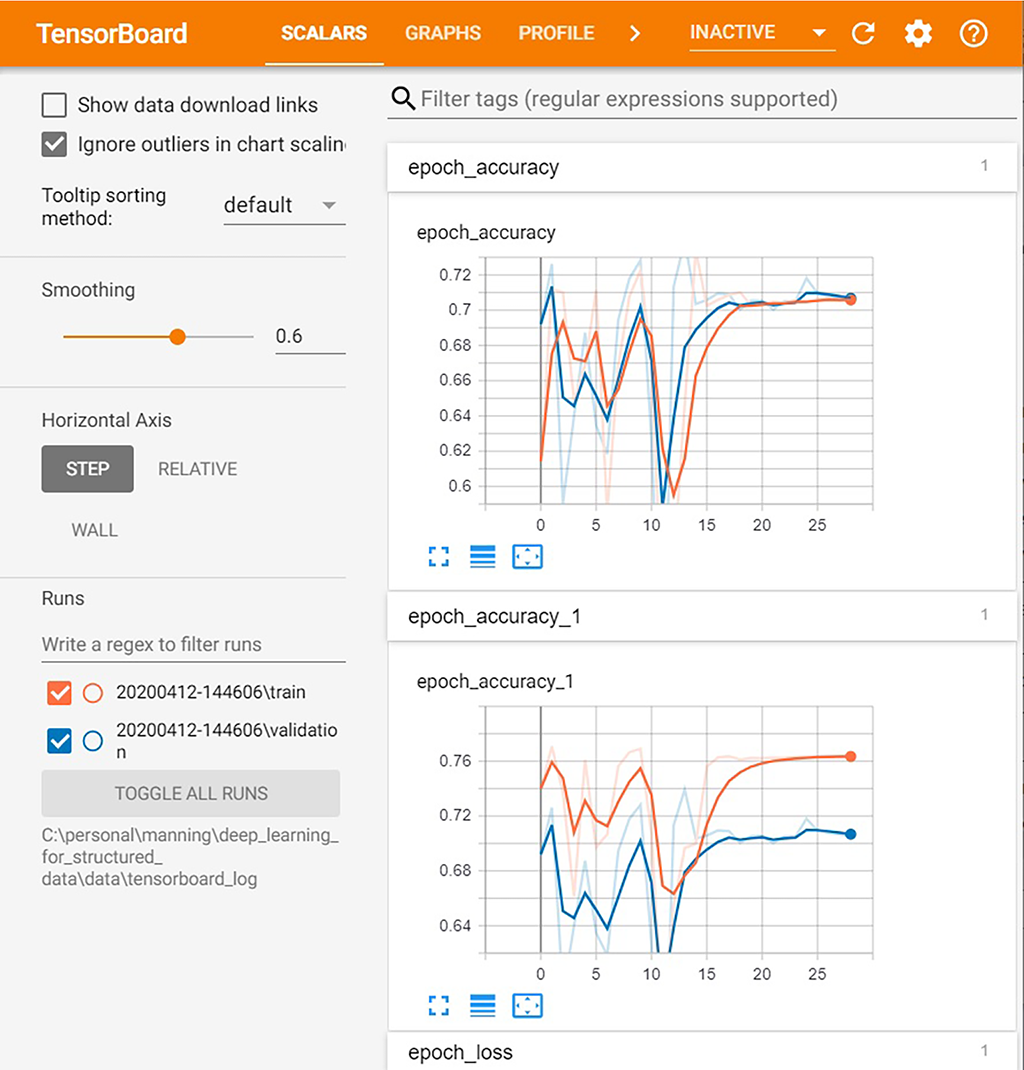
Figure 5.27 TensorBoard showing model accuracy

In this section, you’ve seen three options for getting information about your model: model .summary() , plot_model , and TensorBoard. TensorBoard in particular has a rich set of features for exploring your model. You can get a detailed description of the many visualization options for TensorBoard in the TensorFlow documentation (https://www.tensorflow.org/tensorboard/get_started).

5.15 Model parameters

The code includes a set of parameters that control the operation of the model and its training process. Figure 5.28 summarizes the valid values and purposes of these parameters. A detailed description of the standard parameters (including learning rate, loss function, activation function, batch size, and number of epochs) is beyond the scope of this book. You can find a succinct summary of the key hyperparameters at http://mng.bz/Ov8P.

You can use the parameters listed in figure 5.28 to adjust the behavior of the model. If you are adapting this model to a different dataset, you may want to begin with a smaller learning rate until you get an idea of whether the model is converging on a good result. You will also want to reduce the number of epochs for your first few iterations of training the model on a new dataset until you get an idea of how long it takes for an epoch to complete on your dataset in your training environment.

The output_activation parameter controls whether the model predicts a category (such as streetcar trip delayed/streetcar trip not delayed) or a continuous value (such as “streetcar trip delayed by 5 minutes”). Given the size of the input dataset for streetcar delays, I chose a category prediction for the model. But if you adapt this model for a different dataset, as described in chapter 9, you may decide to use a continuous prediction, and you can adjust the output_activation parameter to a value for a continuous prediction, such as linear.

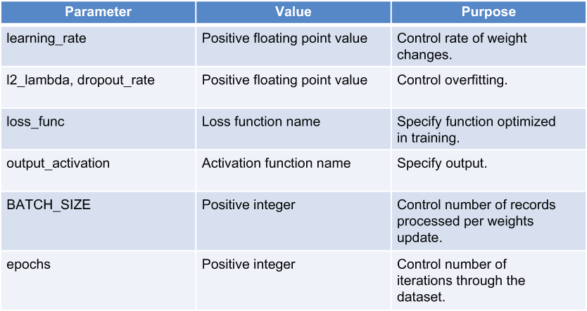
Figure 5.28 Parameters you can set in the code to control the model and its training

These parameters are defined in the config file streetcar_model_training_config.yml. Chapter 3 introduced config files with Python as a way to keep hardcoded values out of your code and to make adjusting parameters faster and less error-prone. The excellent article at http://mng.bz/wpBa has a good description of the value of config files.

You would need to change the parameters listed in figure 5.28 rarely, if at all, when you are going through training iterations. Here’s what these parameters control:

• Learning rate controls the magnitude of changes to the weights per iteration during training of a model. If the learning rate is too high, you can end up skipping the optimal weights, and if it’s too low, progress toward the optimal weights can be extremely slow. The learning rate value that is originally set in the code should be adequate, but you can adjust this value to see how it affects the progress of training of the model.

• Dropout rate controls the proportion of the network that is omitted in training iterations. As we mentioned in section 5.11, with dropout rotating, random subsets of nodes in the network are ignored in forward and backward passes through the network to reduce overfitting.

• L2_lambda controls regularization of the GRU RNN layer. This parameter affects only text input columns. Regularization constrains the weights in the model to reduce overfitting. By forcing down the size of the weights, regularization prevents the model from being influenced too much by particular characteristics of the training set. You can think of regularization as making the model more conservative (https://arxiv.org/ftp/arxiv/papers/2003/2003.05182.pdf) or simpler.

• Loss function is the function that is optimized by the model. The goal of the model is to optimize this function to lead to the best predictions from the model. You can see a comprehensive description of the choices for loss functions available with Keras at http://mng.bz/qNM6. The streetcar delay model predicts a binary choice (whether or not there will be a delay on a particular trip), so binary_crossentropy is the default choice for the loss function.

• Output activation is the function in the final layer of the model that generates the final output. The default setting for this value, hard_sigmoid , will generate output between 0 and 1.

• Batch size is the number of records processed before the model is updated. You should not need to update this value.

• Epochs is the number of complete passes through the training sample. You can adjust this value, starting with a small value to get initial results and then increasing the value if you see better results with a larger number of epochs. Depending on how long it takes to run a single epoch, you may need to balance the additional model performance from more epochs against the time taken to run more epochs.

For the two parameters that define the loss function and the output activation function, Deep Learning with Python contains a useful section (http://mng.bz/7GX7) that goes into greater detail on the options for these parameters and the kinds of problems to which you would apply those options.

Summary

• The code that makes up a deep learning model can be deceptively anticlimactic, but it is the heart of a complete solution that has a raw dataset coming in one end and a deployed trained model coming out the other end.

• Before training a deep learning model with a structured dataset, we need to confirm that all the columns on which the model will be trained will be available at scoring time. If we train the model on data that we won’t have when we want to make a prediction with the model, we risk getting overly optimistic training performance for the model and ending up with a model that cannot generate useful predictions.

• The Keras deep learning model needs to be trained on the data formatted as a list of numpy arrays, so the dataset needs to be transformed from a Pandas dataframe to a list of numpy arrays.

• TensorFlow and Keras began as separate but related projects. Beginning with TensorFlow 2.0, Keras has become the official high-level API for TensorFlow, and its recommended libraries are packaged as part of TensorFlow.

• The Keras functional API combines ease of use with flexibility and is the Keras API that we use for the streetcar delay prediction model.

• The layers of the streetcar delay prediction model are generated automatically based on the categories of the columns: continuous, categorical, and text.

• Embeddings are a powerful concept adapted from the world of natural language processing. With embeddings, you associate vectors with non-numeric values such as the values in categorical columns. The benefits of using embeddings include the ability to manipulate non-numeric values that are analogous to common numeric operations, the ability to get unsupervised learning-type categorization on values in a categorical range as a byproduct of solving a supervised learning problem, and the ability to avoid the drawbacks of one-hot encoding (the other common approach to assigning numeric values to non-numeric tokens).

• You can use a variety of approaches to explore your Keras deep learning model, including model.summary() (for a tabular view), plot_model (for a graphical view), and TensorBoard (for an interactive dashboard).

• You control the behavior of the Keras deep learning model and its training process through a set of parameters. For the streetcar delay prediction model, these parameters are defined in the streetcar_model_training_config.yml config file.