The Birth of NoSQL

Now, in the 2010s, NoSQL is the latest attempt to overthrow the relational model’s dominance. The name “NoSQL” is unfortunate, since it doesn’t actually refer to any particular technology—it was originally intended simply as a catchy Twitter hashtag for a meetup on open source, distributed, nonrelational databases in 2009 [3]. Nevertheless, the term struck a nerve and quickly spread through the web startup community and beyond. A number of interesting database systems are now associated with the #NoSQL hashtag, and it has been retroactively reinterpreted as Not Only SQL [4].

There are several driving forces behind the adoption of NoSQL databases, including:

• A need for greater scalability than relational databases can easily achieve, including very large datasets or very high write throughput

• A widespread preference for free and open source software over commercial database products

• Specialized query operations that are not well supported by the relational model

• Frustration with the restrictiveness of relational schemas, and a desire for a more dynamic and expressive data model [5]

Different applications have different requirements, and the best choice of technology for one use case may well be different from the best choice for another use case. It therefore seems likely that in the foreseeable future, relational databases will continue to be used alongside a broad variety of nonrelational datastores—an idea that is sometimes called polyglot persistence [3].

The Object-Relational Mismatch

Most application development today is done in object-oriented programming languages, which leads to a common criticism of the SQL data model: if data is stored in relational tables, an awkward translation layer is required between the objects in the application code and the database model of tables, rows, and columns. The disconnect between the models is sometimes called an impedance mismatch.ⁱ

Object-relational mapping (ORM) frameworks like ActiveRecord and Hibernate reduce the amount of boilerplate code required for this translation layer, but they can’t completely hide the differences between the two models.

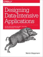
For example, Figure 2-1 illustrates how a résumé (a LinkedIn profile) could be expressed in a relational schema. The profile as a whole can be identified by a unique identifier, user_id. Fields like first_name and last_name appear exactly once per user, so they can be modeled as columns on the users table. However, most people have had more than one job in their career (positions), and people may have varying numbers of periods of education and any number of pieces of contact information. There is a one-to-many relationship from the user to these items, which can be represented in various ways:

• In the traditional SQL model (prior to SQL:1999), the most common normalized representation is to put positions, education, and contact information in separate tables, with a foreign key reference to the users table, as in Figure 2-1.

• Later versions of the SQL standard added support for structured datatypes and XML data; this allowed multi-valued data to be stored within a single row, with support for querying and indexing inside those documents. These features are supported to varying degrees by Oracle, IBM DB2, MS SQL Server, and PostgreSQL [6, 7]. A JSON datatype is also supported by several databases, including IBM DB2, MySQL, and PostgreSQL [8].

• A third option is to encode jobs, education, and contact info as a JSON or XML document, store it on a text column in the database, and let the application interpret its structure and content. In this setup, you typically cannot use the database to query for values inside that encoded column.

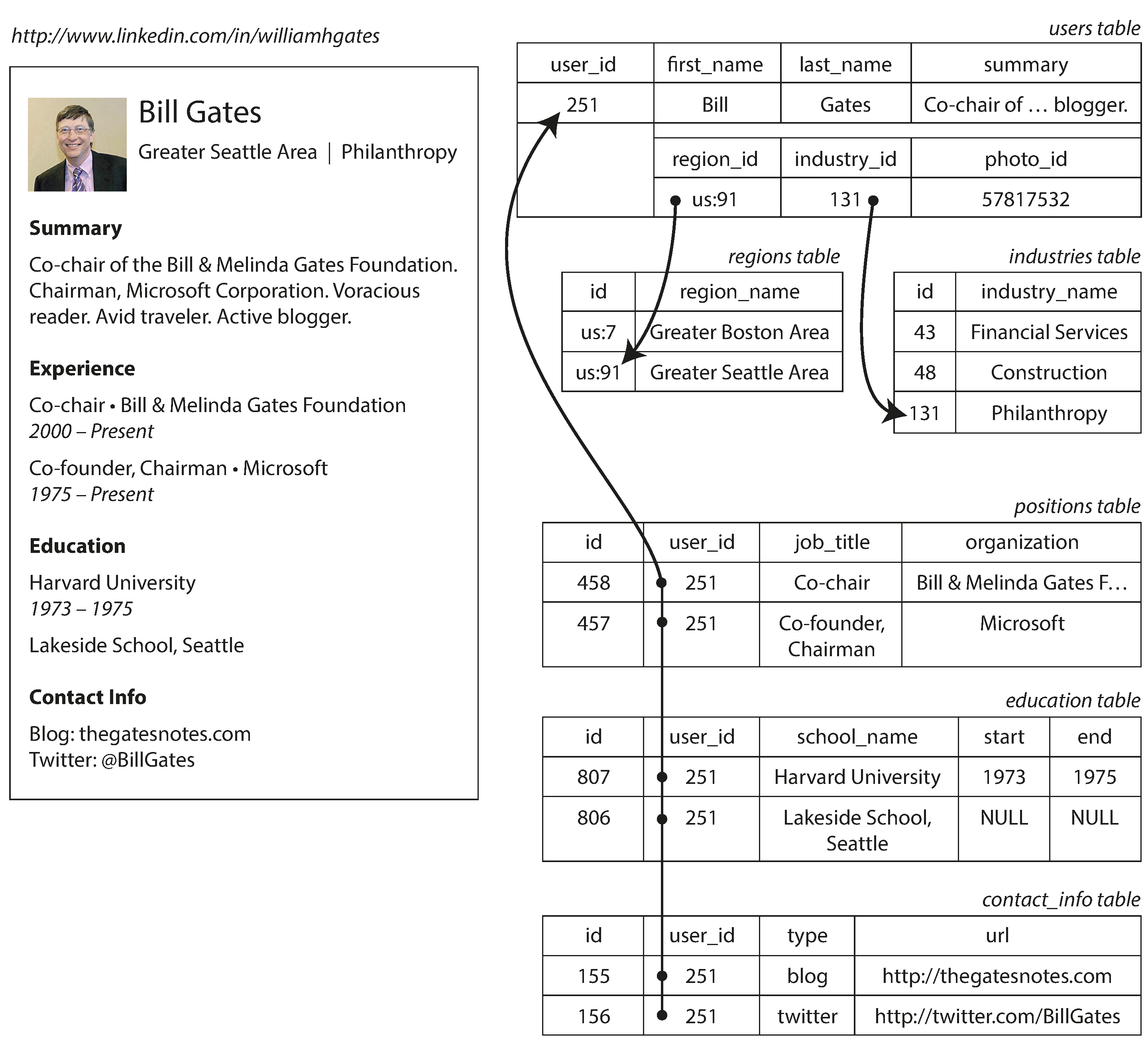
Figure 2-1. Representing a LinkedIn profile using a relational schema. Photo of Bill Gates courtesy of Wikimedia Commons, Ricardo Stuckert, Agência Brasil.

For a data structure like a résumé, which is mostly a self-contained document, a JSON representation can be quite appropriate: see Example 2-1. JSON has the appeal of being much simpler than XML. Document-oriented databases like MongoDB [9], RethinkDB [10], CouchDB [11], and Espresso [12] support this data model.

{
  "user_id":     251,
  "first_name":  "Bill",
  "last_name":   "Gates",
  "summary":     "Co-chair of the Bill & Melinda Gates... Active blogger.",
  "region_id":   "us:91",
  "industry_id": 131,
  "photo_url":   "/p/7/000/253/05b/308dd6e.jpg",
  "positions": [
    {"job_title": "Co-chair", "organization": "Bill & Melinda Gates Foundation"},
    {"job_title": "Co-founder, Chairman", "organization": "Microsoft"}
  ],
  "education": [
    {"school_name": "Harvard University",       "start": 1973, "end": 1975},
    {"school_name": "Lakeside School, Seattle", "start": null, "end": null}
  ],
  "contact_info": {
    "blog":    "http://thegatesnotes.com",
    "twitter": "http://twitter.com/BillGates"
  }
}

Some developers feel that the JSON model reduces the impedance mismatch between the application code and the storage layer. However, as we shall see in Chapter 4, there are also problems with JSON as a data encoding format. The lack of a schema is often cited as an advantage; we will discuss this in “Schema flexibility in the document model”.

The JSON representation has better locality than the multi-table schema in Figure 2-1. If you want to fetch a profile in the relational example, you need to either perform multiple queries (query each table by user_id) or perform a messy multi-way join between the users table and its subordinate tables. In the JSON representation, all the relevant information is in one place, and one query is sufficient.

The one-to-many relationships from the user profile to the user’s positions, educational history, and contact information imply a tree structure in the data, and the JSON representation makes this tree structure explicit (see Figure 2-2).

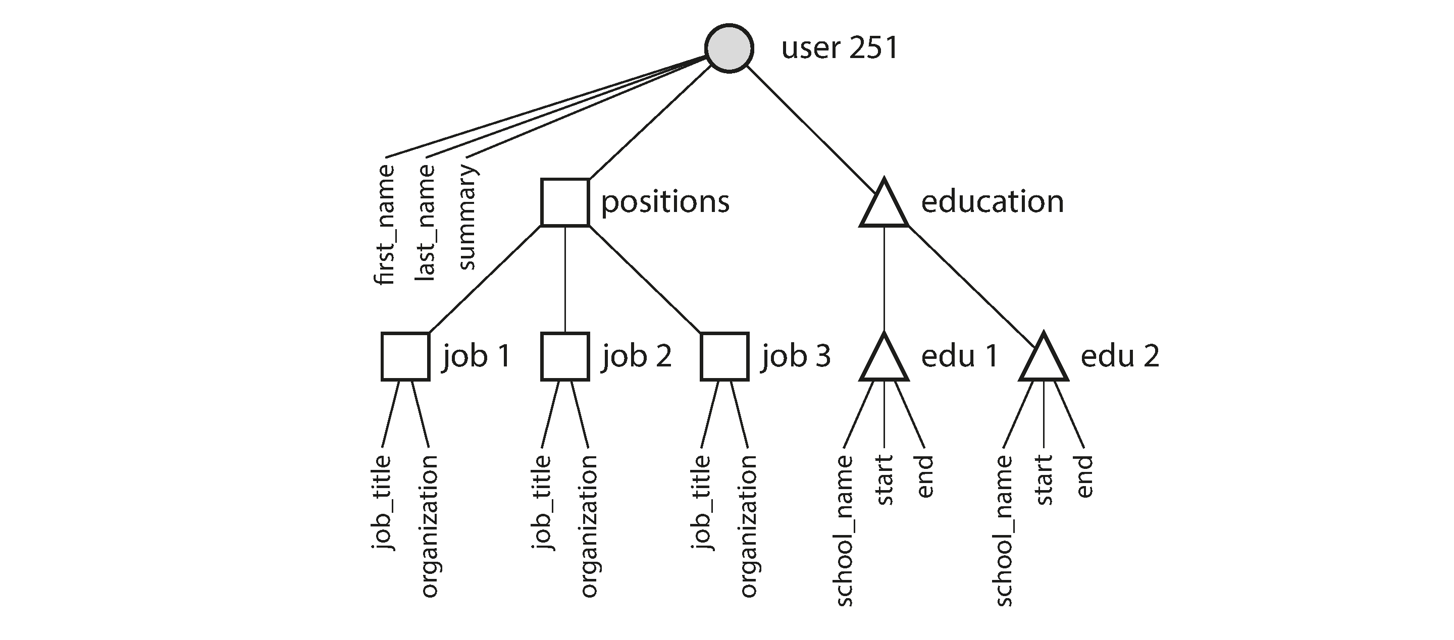
Figure 2-2. One-to-many relationships forming a tree structure.

Many-to-One and Many-to-Many Relationships

In Example 2-1 in the preceding section, region_id and industry_id are given as IDs, not as plain-text strings "Greater Seattle Area" and "Philanthropy". Why?

If the user interface has free-text fields for entering the region and the industry, it makes sense to store them as plain-text strings. But there are advantages to having standardized lists of geographic regions and industries, and letting users choose from a drop-down list or autocompleter:

• Consistent style and spelling across profiles

• Avoiding ambiguity (e.g., if there are several cities with the same name)

• Ease of updating—the name is stored in only one place, so it is easy to update across the board if it ever needs to be changed (e.g., change of a city name due to political events)

• Localization support—when the site is translated into other languages, the standardized lists can be localized, so the region and industry can be displayed in the viewer’s language

• Better search—e.g., a search for philanthropists in the state of Washington can match this profile, because the list of regions can encode the fact that Seattle is in Washington (which is not apparent from the string "Greater Seattle Area")

Whether you store an ID or a text string is a question of duplication. When you use an ID, the information that is meaningful to humans (such as the word Philanthropy) is stored in only one place, and everything that refers to it uses an ID (which only has meaning within the database). When you store the text directly, you are duplicating the human-meaningful information in every record that uses it.

The advantage of using an ID is that because it has no meaning to humans, it never needs to change: the ID can remain the same, even if the information it identifies changes. Anything that is meaningful to humans may need to change sometime in the future—and if that information is duplicated, all the redundant copies need to be updated. That incurs write overheads, and risks inconsistencies (where some copies of the information are updated but others aren’t). Removing such duplication is the key idea behind normalization in databases.ⁱⁱ

Unfortunately, normalizing this data requires many-to-one relationships (many people live in one particular region, many people work in one particular industry), which don’t fit nicely into the document model. In relational databases, it’s normal to refer to rows in other tables by ID, because joins are easy. In document databases, joins are not needed for one-to-many tree structures, and support for joins is often weak.ⁱⁱⁱ

If the database itself does not support joins, you have to emulate a join in application code by making multiple queries to the database. (In this case, the lists of regions and industries are probably small and slow-changing enough that the application can simply keep them in memory. But nevertheless, the work of making the join is shifted from the database to the application code.)

Moreover, even if the initial version of an application fits well in a join-free document model, data has a tendency of becoming more interconnected as features are added to applications. For example, consider some changes we could make to the résumé example:

Organizations and schools as entities

In the previous description, organization (the company where the user worked) and school_name (where they studied) are just strings. Perhaps they should be references to entities instead? Then each organization, school, or university could have its own web page (with logo, news feed, etc.); each résumé could link to the organizations and schools that it mentions, and include their logos and other information (see Figure 2-3 for an example from LinkedIn).

Recommendations

Say you want to add a new feature: one user can write a recommendation for another user. The recommendation is shown on the résumé of the user who was recommended, together with the name and photo of the user making the recommendation. If the recommender updates their photo, any recommendations they have written need to reflect the new photo. Therefore, the recommendation should have a reference to the author’s profile.

Figure 2-3. The company name is not just a string, but a link to a company entity. Screenshot of linkedin.com.

Figure 2-4 illustrates how these new features require many-to-many relationships. The data within each dotted rectangle can be grouped into one document, but the references to organizations, schools, and other users need to be represented as references, and require joins when queried.

Figure 2-4. Extending résumés with many-to-many relationships.

Are Document Databases Repeating History?

While many-to-many relationships and joins are routinely used in relational databases, document databases and NoSQL reopened the debate on how best to represent such relationships in a database. This debate is much older than NoSQL—in fact, it goes back to the very earliest computerized database systems.

The most popular database for business data processing in the 1970s was IBM’s Information Management System (IMS), originally developed for stock-keeping in the Apollo space program and first commercially released in 1968 [13]. It is still in use and maintained today, running on OS/390 on IBM mainframes [14].

The design of IMS used a fairly simple data model called the hierarchical model, which has some remarkable similarities to the JSON model used by document databases [2]. It represented all data as a tree of records nested within records, much like the JSON structure of Figure 2-2.

Like document databases, IMS worked well for one-to-many relationships, but it made many-to-many relationships difficult, and it didn’t support joins. Developers had to decide whether to duplicate (denormalize) data or to manually resolve references from one record to another. These problems of the 1960s and ’70s were very much like the problems that developers are running into with document databases today [15].

Various solutions were proposed to solve the limitations of the hierarchical model. The two most prominent were the relational model (which became SQL, and took over the world) and the network model (which initially had a large following but eventually faded into obscurity). The “great debate” between these two camps lasted for much of the 1970s [2].

Since the problem that the two models were solving is still so relevant today, it’s worth briefly revisiting this debate in today’s light.

Relational Versus Document Databases Today

There are many differences to consider when comparing relational databases to document databases, including their fault-tolerance properties (see Chapter 5) and handling of concurrency (see Chapter 7). In this chapter, we will concentrate only on the differences in the data model.

The main arguments in favor of the document data model are schema flexibility, better performance due to locality, and that for some applications it is closer to the data structures used by the application. The relational model counters by providing better support for joins, and many-to-one and many-to-many relationships.

if (user && user.name && !user.first_name) {
    // Documents written before Dec 8, 2013 don't have first_name
    user.first_name = user.name.split(" ")[0];
}

ALTER TABLE users ADD COLUMN first_name text;
UPDATE users SET first_name = split_part(name, ' ', 1);      -- PostgreSQL
UPDATE users SET first_name = substring_index(name, ' ', 1);      -- MySQL

Declarative Queries on the Web

The advantages of declarative query languages are not limited to just databases. To illustrate the point, let’s compare declarative and imperative approaches in a completely different environment: a web browser.

Say you have a website about animals in the ocean. The user is currently viewing the page on sharks, so you mark the navigation item “Sharks” as currently selected, like this:

<ul>
    <li class="selected"> 
        <p>Sharks</p> 
        <ul>
            <li>Great White Shark</li>
            <li>Tiger Shark</li>
            <li>Hammerhead Shark</li>
        </ul>
    </li>
    <li>
        <p>Whales</p>
        <ul>
            <li>Blue Whale</li>
            <li>Humpback Whale</li>
            <li>Fin Whale</li>
        </ul>
    </li>
</ul>

The selected item is marked with the CSS class "selected".

<p>Sharks</p> is the title of the currently selected page.

Now say you want the title of the currently selected page to have a blue background, so that it is visually highlighted. This is easy, using CSS:

li.selected > p {
    background-color: blue;
}

Here the CSS selector li.selected > p declares the pattern of elements to which we want to apply the blue style: namely, all <p> elements whose direct parent is an <li> element with a CSS class of selected. The element <p>Sharks</p> in the example matches this pattern, but <p>Whales</p> does not match because its <li> parent lacks class="selected".

If you were using XSL instead of CSS, you could do something similar:

<xsl:template match="li[@class='selected']/p">
    <fo:block background-color="blue">
        <xsl:apply-templates/>
    </fo:block>
</xsl:template>

Here, the XPath expression li[@class='selected']/p is equivalent to the CSS selector li.selected > p in the previous example. What CSS and XSL have in common is that they are both declarative languages for specifying the styling of a document.

Imagine what life would be like if you had to use an imperative approach. In JavaScript, using the core Document Object Model (DOM) API, the result might look something like this:

var liElements = document.getElementsByTagName("li");
for (var i = 0; i < liElements.length; i++) {
    if (liElements[i].className === "selected") {
        var children = liElements[i].childNodes;
        for (var j = 0; j < children.length; j++) {
            var child = children[j];
            if (child.nodeType === Node.ELEMENT_NODE && child.tagName === "P") {
                child.setAttribute("style", "background-color: blue");
            }
        }
    }
}

This JavaScript imperatively sets the element <p>Sharks</p> to have a blue background, but the code is awful. Not only is it much longer and harder to understand than the CSS and XSL equivalents, but it also has some serious problems:

• If the selected class is removed (e.g., because the user clicks a different page), the blue color won’t be removed, even if the code is rerun—and so the item will remain highlighted until the entire page is reloaded. With CSS, the browser automatically detects when the li.selected > p rule no longer applies and removes the blue background as soon as the selected class is removed.

• If you want to take advantage of a new API, such as document.getElementsByClassName("selected") or even document.evaluate()—which may improve performance—you have to rewrite the code. On the other hand, browser vendors can improve the performance of CSS and XPath without breaking compatibility.

In a web browser, using declarative CSS styling is much better than manipulating styles imperatively in JavaScript. Similarly, in databases, declarative query languages like SQL turned out to be much better than imperative query APIs.^vi

MapReduce Querying

MapReduce is a programming model for processing large amounts of data in bulk across many machines, popularized by Google [33]. A limited form of MapReduce is supported by some NoSQL datastores, including MongoDB and CouchDB, as a mechanism for performing read-only queries across many documents.

MapReduce in general is described in more detail in Chapter 10. For now, we’ll just briefly discuss MongoDB’s use of the model.

MapReduce is neither a declarative query language nor a fully imperative query API, but somewhere in between: the logic of the query is expressed with snippets of code, which are called repeatedly by the processing framework. It is based on the map (also known as collect) and reduce (also known as fold or inject) functions that exist in many functional programming languages.

To give an example, imagine you are a marine biologist, and you add an observation record to your database every time you see animals in the ocean. Now you want to generate a report saying how many sharks you have sighted per month.

In PostgreSQL you might express that query like this:

SELECT date_trunc('month', observation_timestamp) AS observation_month, 
       sum(num_animals) AS total_animals
FROM observations
WHERE family = 'Sharks'
GROUP BY observation_month;

The date_trunc('month', timestamp) function determines the calendar month containing timestamp, and returns another timestamp representing the beginning of that month. In other words, it rounds a timestamp down to the nearest month.

This query first filters the observations to only show species in the Sharks family, then groups the observations by the calendar month in which they occurred, and finally adds up the number of animals seen in all observations in that month.

The same can be expressed with MongoDB’s MapReduce feature as follows:

db.observations.mapReduce(
    function map() { 
        var year  = this.observationTimestamp.getFullYear();
        var month = this.observationTimestamp.getMonth() + 1;
        emit(year + "-" + month, this.numAnimals); 
    },
    function reduce(key, values) { 
        return Array.sum(values); 
    },
    {
        query: { family: "Sharks" }, 
        out: "monthlySharkReport" 
    }
);

The filter to consider only shark species can be specified declaratively (this is a MongoDB-specific extension to MapReduce).

The JavaScript function map is called once for every document that matches query, with this set to the document object.

The map function emits a key (a string consisting of year and month, such as "2013-12" or "2014-1") and a value (the number of animals in that observation).

The key-value pairs emitted by map are grouped by key. For all key-value pairs with the same key (i.e., the same month and year), the reduce function is called once.

The reduce function adds up the number of animals from all observations in a particular month.

The final output is written to the collection monthlySharkReport.

For example, say the observations collection contains these two documents:

{
    observationTimestamp: Date.parse("Mon, 25 Dec 1995 12:34:56 GMT"),
    family:     "Sharks",
    species:    "Carcharodon carcharias",
    numAnimals: 3
}
{
    observationTimestamp: Date.parse("Tue, 12 Dec 1995 16:17:18 GMT"),
    family:     "Sharks",
    species:    "Carcharias taurus",
    numAnimals: 4
}

The map function would be called once for each document, resulting in emit("1995-12", 3) and emit("1995-12", 4). Subsequently, the reduce function would be called with reduce("1995-12", [3, 4]), returning 7.

The map and reduce functions are somewhat restricted in what they are allowed to do. They must be pure functions, which means they only use the data that is passed to them as input, they cannot perform additional database queries, and they must not have any side effects. These restrictions allow the database to run the functions anywhere, in any order, and rerun them on failure. However, they are nevertheless powerful: they can parse strings, call library functions, perform calculations, and more.

MapReduce is a fairly low-level programming model for distributed execution on a cluster of machines. Higher-level query languages like SQL can be implemented as a pipeline of MapReduce operations (see Chapter 10), but there are also many distributed implementations of SQL that don’t use MapReduce. Note there is nothing in SQL that constrains it to running on a single machine, and MapReduce doesn’t have a monopoly on distributed query execution.

Being able to use JavaScript code in the middle of a query is a great feature for advanced queries, but it’s not limited to MapReduce—some SQL databases can be extended with JavaScript functions too [34].

A usability problem with MapReduce is that you have to write two carefully coordinated JavaScript functions, which is often harder than writing a single query. Moreover, a declarative query language offers more opportunities for a query optimizer to improve the performance of a query. For these reasons, MongoDB 2.2 added support for a declarative query language called the aggregation pipeline [9]. In this language, the same shark-counting query looks like this:

db.observations.aggregate([
    { $match: { family: "Sharks" } },
    { $group: {
        _id: {
            year:  { $year:  "$observationTimestamp" },
            month: { $month: "$observationTimestamp" }
        },
        totalAnimals: { $sum: "$numAnimals" }
    } }
]);

The aggregation pipeline language is similar in expressiveness to a subset of SQL, but it uses a JSON-based syntax rather than SQL’s English-sentence-style syntax; the difference is perhaps a matter of taste. The moral of the story is that a NoSQL system may find itself accidentally reinventing SQL, albeit in disguise.

Property Graphs

In the property graph model, each vertex consists of:

• A unique identifier

• A set of outgoing edges

• A set of incoming edges

• A collection of properties (key-value pairs)

Each edge consists of:

• A unique identifier

• The vertex at which the edge starts (the tail vertex)

• The vertex at which the edge ends (the head vertex)

• A label to describe the kind of relationship between the two vertices

• A collection of properties (key-value pairs)

You can think of a graph store as consisting of two relational tables, one for vertices and one for edges, as shown in Example 2-2 (this schema uses the PostgreSQL json datatype to store the properties of each vertex or edge). The head and tail vertex are stored for each edge; if you want the set of incoming or outgoing edges for a vertex, you can query the edges table by head_vertex or tail_vertex, respectively.

CREATE TABLE vertices (
    vertex_id   integer PRIMARY KEY,
    properties  json
);

CREATE TABLE edges (
    edge_id     integer PRIMARY KEY,
    tail_vertex integer REFERENCES vertices (vertex_id),
    head_vertex integer REFERENCES vertices (vertex_id),
    label       text,
    properties  json
);

CREATE INDEX edges_tails ON edges (tail_vertex);
CREATE INDEX edges_heads ON edges (head_vertex);

Some important aspects of this model are:

1. Any vertex can have an edge connecting it with any other vertex. There is no schema that restricts which kinds of things can or cannot be associated.

2. Given any vertex, you can efficiently find both its incoming and its outgoing edges, and thus traverse the graph—i.e., follow a path through a chain of vertices—both forward and backward. (That’s why Example 2-2 has indexes on both the tail_vertex and head_vertex columns.)

3. By using different labels for different kinds of relationships, you can store several different kinds of information in a single graph, while still maintaining a clean data model.

Those features give graphs a great deal of flexibility for data modeling, as illustrated in Figure 2-5. The figure shows a few things that would be difficult to express in a traditional relational schema, such as different kinds of regional structures in different countries (France has départements and régions, whereas the US has counties and states), quirks of history such as a country within a country (ignoring for now the intricacies of sovereign states and nations), and varying granularity of data (Lucy’s current residence is specified as a city, whereas her place of birth is specified only at the level of a state).

You could imagine extending the graph to also include many other facts about Lucy and Alain, or other people. For instance, you could use it to indicate any food allergies they have (by introducing a vertex for each allergen, and an edge between a person and an allergen to indicate an allergy), and link the allergens with a set of vertices that show which foods contain which substances. Then you could write a query to find out what is safe for each person to eat. Graphs are good for evolvability: as you add features to your application, a graph can easily be extended to accommodate changes in your application’s data structures.

The Cypher Query Language

Cypher is a declarative query language for property graphs, created for the Neo4j graph database [37]. (It is named after a character in the movie The Matrix and is not related to ciphers in cryptography [38].)

Example 2-3 shows the Cypher query to insert the lefthand portion of Figure 2-5 into a graph database. The rest of the graph can be added similarly and is omitted for readability. Each vertex is given a symbolic name like USA or Idaho, and other parts of the query can use those names to create edges between the vertices, using an arrow notation: (Idaho) -[:WITHIN]-> (USA) creates an edge labeled WITHIN, with Idaho as the tail node and USA as the head node.

CREATE
  (NAmerica:Location {name:'North America', type:'continent'}),
  (USA:Location      {name:'United States', type:'country'  }),
  (Idaho:Location    {name:'Idaho',         type:'state'    }),
  (Lucy:Person       {name:'Lucy' }),
  (Idaho) -[:WITHIN]->  (USA)  -[:WITHIN]-> (NAmerica),
  (Lucy)  -[:BORN_IN]-> (Idaho)

When all the vertices and edges of Figure 2-5 are added to the database, we can start asking interesting questions: for example, find the names of all the people who emigrated from the United States to Europe. To be more precise, here we want to find all the vertices that have a BORN_IN edge to a location within the US, and also a LIVING_IN edge to a location within Europe, and return the name property of each of those vertices.

Example 2-4 shows how to express that query in Cypher. The same arrow notation is used in a MATCH clause to find patterns in the graph: (person) -[:BORN_IN]-> () matches any two vertices that are related by an edge labeled BORN_IN. The tail vertex of that edge is bound to the variable person, and the head vertex is left unnamed.

MATCH
  (person) -[:BORN_IN]->  () -[:WITHIN*0..]-> (us:Location {name:'United States'}),
  (person) -[:LIVES_IN]-> () -[:WITHIN*0..]-> (eu:Location {name:'Europe'})
RETURN person.name

The query can be read as follows:

Find any vertex (call it person) that meets both of the following conditions:

1. person has an outgoing BORN_IN edge to some vertex. From that vertex, you can follow a chain of outgoing WITHIN edges until eventually you reach a vertex of type Location, whose name property is equal to "United States".

2. That same person vertex also has an outgoing LIVES_IN edge. Following that edge, and then a chain of outgoing WITHIN edges, you eventually reach a vertex of type Location, whose name property is equal to "Europe".

For each such person vertex, return the name property.

There are several possible ways of executing the query. The description given here suggests that you start by scanning all the people in the database, examine each person’s birthplace and residence, and return only those people who meet the criteria.

But equivalently, you could start with the two Location vertices and work backward. If there is an index on the name property, you can probably efficiently find the two vertices representing the US and Europe. Then you can proceed to find all locations (states, regions, cities, etc.) in the US and Europe respectively by following all incoming WITHIN edges. Finally, you can look for people who can be found through an incoming BORN_IN or LIVES_IN edge at one of the location vertices.

As is typical for a declarative query language, you don’t need to specify such execution details when writing the query: the query optimizer automatically chooses the strategy that is predicted to be the most efficient, so you can get on with writing the rest of your application.

Graph Queries in SQL

Example 2-2 suggested that graph data can be represented in a relational database. But if we put graph data in a relational structure, can we also query it using SQL?

The answer is yes, but with some difficulty. In a relational database, you usually know in advance which joins you need in your query. In a graph query, you may need to traverse a variable number of edges before you find the vertex you’re looking for—that is, the number of joins is not fixed in advance.

In our example, that happens in the () -[:WITHIN*0..]-> () rule in the Cypher query. A person’s LIVES_IN edge may point at any kind of location: a street, a city, a district, a region, a state, etc. A city may be WITHIN a region, a region WITHIN a state, a state WITHIN a country, etc. The LIVES_IN edge may point directly at the location vertex you’re looking for, or it may be several levels removed in the location hierarchy.

In Cypher, :WITHIN*0.. expresses that fact very concisely: it means “follow a WITHIN edge, zero or more times.” It is like the * operator in a regular expression.

Since SQL:1999, this idea of variable-length traversal paths in a query can be expressed using something called recursive common table expressions (the WITH RECURSIVE syntax). Example 2-5 shows the same query—finding the names of people who emigrated from the US to Europe—expressed in SQL using this technique (supported in PostgreSQL, IBM DB2, Oracle, and SQL Server). However, the syntax is very clumsy in comparison to Cypher.

WITH RECURSIVE

  -- in_usa is the set of vertex IDs of all locations within the United States
  in_usa(vertex_id) AS (
      SELECT vertex_id FROM vertices WHERE properties->>'name' = 'United States' 
    UNION
      SELECT edges.tail_vertex FROM edges 
        JOIN in_usa ON edges.head_vertex = in_usa.vertex_id
        WHERE edges.label = 'within'
  ),

  -- in_europe is the set of vertex IDs of all locations within Europe
  in_europe(vertex_id) AS (
      SELECT vertex_id FROM vertices WHERE properties->>'name' = 'Europe' 
    UNION
      SELECT edges.tail_vertex FROM edges
        JOIN in_europe ON edges.head_vertex = in_europe.vertex_id
        WHERE edges.label = 'within'
  ),

  -- born_in_usa is the set of vertex IDs of all people born in the US
  born_in_usa(vertex_id) AS ( 
    SELECT edges.tail_vertex FROM edges
      JOIN in_usa ON edges.head_vertex = in_usa.vertex_id
      WHERE edges.label = 'born_in'
  ),

  -- lives_in_europe is the set of vertex IDs of all people living in Europe
  lives_in_europe(vertex_id) AS ( 
    SELECT edges.tail_vertex FROM edges
      JOIN in_europe ON edges.head_vertex = in_europe.vertex_id
      WHERE edges.label = 'lives_in'
  )

SELECT vertices.properties->>'name'
FROM vertices
-- join to find those people who were both born in the US *and* live in Europe
JOIN born_in_usa     ON vertices.vertex_id = born_in_usa.vertex_id 
JOIN lives_in_europe ON vertices.vertex_id = lives_in_europe.vertex_id;

If the same query can be written in 4 lines in one query language but requires 29 lines in another, that just shows that different data models are designed to satisfy different use cases. It’s important to pick a data model that is suitable for your application.

Triple-Stores and SPARQL

The triple-store model is mostly equivalent to the property graph model, using different words to describe the same ideas. It is nevertheless worth discussing, because there are various tools and languages for triple-stores that can be valuable additions to your toolbox for building applications.

In a triple-store, all information is stored in the form of very simple three-part statements: (subject, predicate, object). For example, in the triple (Jim, likes, bananas), Jim is the subject, likes is the predicate (verb), and bananas is the object.

The subject of a triple is equivalent to a vertex in a graph. The object is one of two things:

1. A value in a primitive datatype, such as a string or a number. In that case, the predicate and object of the triple are equivalent to the key and value of a property on the subject vertex. For example, (lucy, age, 33) is like a vertex lucy with properties {"age":33}.

2. Another vertex in the graph. In that case, the predicate is an edge in the graph, the subject is the tail vertex, and the object is the head vertex. For example, in (lucy, marriedTo, alain) the subject and object lucy and alain are both vertices, and the predicate marriedTo is the label of the edge that connects them.

Example 2-6 shows the same data as in Example 2-3, written as triples in a format called Turtle, a subset of Notation3 (N3) [39].

@prefix : <urn:example:>.
_:lucy     a       :Person.
_:lucy     :name   "Lucy".
_:lucy     :bornIn _:idaho.
_:idaho    a       :Location.
_:idaho    :name   "Idaho".
_:idaho    :type   "state".
_:idaho    :within _:usa.
_:usa      a       :Location.
_:usa      :name   "United States".
_:usa      :type   "country".
_:usa      :within _:namerica.
_:namerica a       :Location.
_:namerica :name   "North America".
_:namerica :type   "continent".

In this example, vertices of the graph are written as _:someName. The name doesn’t mean anything outside of this file; it exists only because we otherwise wouldn’t know which triples refer to the same vertex. When the predicate represents an edge, the object is a vertex, as in _:idaho :within _:usa. When the predicate is a property, the object is a string literal, as in _:usa :name "United States".

It’s quite repetitive to repeat the same subject over and over again, but fortunately you can use semicolons to say multiple things about the same subject. This makes the Turtle format quite nice and readable: see Example 2-7.

@prefix : <urn:example:>.
_:lucy     a :Person;   :name "Lucy";          :bornIn _:idaho.
_:idaho    a :Location; :name "Idaho";         :type "state";   :within _:usa.
_:usa      a :Location; :name "United States"; :type "country"; :within _:namerica.
_:namerica a :Location; :name "North America"; :type "continent".

<rdf:RDF xmlns="urn:example:"
    xmlns:rdf="http://www.w3.org/1999/02/22-rdf-syntax-ns#">

  <Location rdf:nodeID="idaho">
    <name>Idaho</name>
    <type>state</type>
    <within>
      <Location rdf:nodeID="usa">
        <name>United States</name>
        <type>country</type>
        <within>
          <Location rdf:nodeID="namerica">
            <name>North America</name>
            <type>continent</type>
          </Location>
        </within>
      </Location>
    </within>
  </Location>

  <Person rdf:nodeID="lucy">
    <name>Lucy</name>
    <bornIn rdf:nodeID="idaho"/>
  </Person>
</rdf:RDF>

PREFIX : <urn:example:>

SELECT ?personName WHERE {
  ?person :name ?personName.
  ?person :bornIn  / :within* / :name "United States".
  ?person :livesIn / :within* / :name "Europe".
}

(person) -[:BORN_IN]-> () -[:WITHIN*0..]-> (location)   # Cypher

?person :bornIn / :within* ?location.                   # SPARQL

(usa {name:'United States'})   # Cypher

?usa :name "United States".    # SPARQL

The Foundation: Datalog

Datalog is a much older language than SPARQL or Cypher, having been studied extensively by academics in the 1980s [44, 45, 46]. It is less well known among software engineers, but it is nevertheless important, because it provides the foundation that later query languages build upon.

In practice, Datalog is used in a few data systems: for example, it is the query language of Datomic [40], and Cascalog [47] is a Datalog implementation for querying large datasets in Hadoop.^viii

Datalog’s data model is similar to the triple-store model, generalized a bit. Instead of writing a triple as (subject, predicate, object), we write it as predicate(subject, object). Example 2-10 shows how to write the data from our example in Datalog.

name(namerica, 'North America').
type(namerica, continent).

name(usa, 'United States').
type(usa, country).
within(usa, namerica).

name(idaho, 'Idaho').
type(idaho, state).
within(idaho, usa).

name(lucy, 'Lucy').
born_in(lucy, idaho).

Now that we have defined the data, we can write the same query as before, as shown in Example 2-11. It looks a bit different from the equivalent in Cypher or SPARQL, but don’t let that put you off. Datalog is a subset of Prolog, which you might have seen before if you’ve studied computer science.

within_recursive(Location, Name) :- name(Location, Name).     /* Rule 1 */

within_recursive(Location, Name) :- within(Location, Via),    /* Rule 2 */
                                    within_recursive(Via, Name).

migrated(Name, BornIn, LivingIn) :- name(Person, Name),       /* Rule 3 */
                                    born_in(Person, BornLoc),
                                    within_recursive(BornLoc, BornIn),
                                    lives_in(Person, LivingLoc),
                                    within_recursive(LivingLoc, LivingIn).

?- migrated(Who, 'United States', 'Europe').
/* Who = 'Lucy'. */

Cypher and SPARQL jump in right away with SELECT, but Datalog takes a small step at a time. We define rules that tell the database about new predicates: here, we define two new predicates, within_recursive and migrated. These predicates aren’t triples stored in the database, but instead they are derived from data or from other rules. Rules can refer to other rules, just like functions can call other functions or recursively call themselves. Like this, complex queries can be built up a small piece at a time.

In rules, words that start with an uppercase letter are variables, and predicates are matched like in Cypher and SPARQL. For example, name(Location, Name) matches the triple name(namerica, 'North America') with variable bindings Location = namerica and Name = 'North America'.

A rule applies if the system can find a match for all predicates on the righthand side of the :- operator. When the rule applies, it’s as though the lefthand side of the :- was added to the database (with variables replaced by the values they matched).

One possible way of applying the rules is thus:

1. name(namerica, 'North America') exists in the database, so rule 1 applies. It generates within_recursive(namerica, 'North America').

2. within(usa, namerica) exists in the database and the previous step generated within_recursive(namerica, 'North America'), so rule 2 applies. It generates within_recursive(usa, 'North America').

3. within(idaho, usa) exists in the database and the previous step generated within_recursive(usa, 'North America'), so rule 2 applies. It generates within_recursive(idaho, 'North America').

By repeated application of rules 1 and 2, the within_recursive predicate can tell us all the locations in North America (or any other location name) contained in our database. This process is illustrated in Figure 2-6.

Figure 2-6. Determining that Idaho is in North America, using the Datalog rules from Example 2-11.

Now rule 3 can find people who were born in some location BornIn and live in some location LivingIn. By querying with BornIn = 'United States' and LivingIn = 'Europe', and leaving the person as a variable Who, we ask the Datalog system to find out which values can appear for the variable Who. So, finally we get the same answer as in the earlier Cypher and SPARQL queries.

The Datalog approach requires a different kind of thinking to the other query languages discussed in this chapter, but it’s a very powerful approach, because rules can be combined and reused in different queries. It’s less convenient for simple one-off queries, but it can cope better if your data is complex.

References

[1] Edgar F. Codd: “A Relational Model of Data for Large Shared Data Banks,” Communications of the ACM, volume 13, number 6, pages 377–387, June 1970. doi:10.1145/362384.362685
[2] Michael Stonebraker and Joseph M. Hellerstein: “What Goes Around Comes Around,” in Readings in Database Systems, 4th edition, MIT Press, pages 2–41, 2005. ISBN: 978-0-262-69314-1
[3] Pramod J. Sadalage and Martin Fowler: NoSQL Distilled. Addison-Wesley, August 2012. ISBN: 978-0-321-82662-6
[4] Eric Evans: “NoSQL: What’s in a Name?,” blog.sym-link.com, October 30, 2009.
[5] James Phillips: “Surprises in Our NoSQL Adoption Survey,” blog.couchbase.com, February 8, 2012.
[6] Michael Wagner: SQL/XML:2006 – Evaluierung der Standardkonformität ausgewählter Datenbanksysteme. Diplomica Verlag, Hamburg, 2010. ISBN: 978-3-836-64609-3
[7] “XML Data in SQL Server,” SQL Server 2012 documentation, technet.microsoft.com, 2013.
[8] “PostgreSQL 9.3.1 Documentation,” The PostgreSQL Global Development Group, 2013.
[9] “The MongoDB 2.4 Manual,” MongoDB, Inc., 2013.
[10] “RethinkDB 1.11 Documentation,” rethinkdb.com, 2013.
[11] “Apache CouchDB 1.6 Documentation,” docs.couchdb.org, 2014.
[12] Lin Qiao, Kapil Surlaker, Shirshanka Das, et al.: “On Brewing Fresh Espresso: LinkedIn’s Distributed Data Serving Platform,” at ACM International Conference on Management of Data (SIGMOD), June 2013.
[13] Rick Long, Mark Harrington, Robert Hain, and Geoff Nicholls: IMS Primer. IBM Redbook SG24-5352-00, IBM International Technical Support Organization, January 2000.
[14] Stephen D. Bartlett: “IBM’s IMS—Myths, Realities, and Opportunities,” The Clipper Group Navigator, TCG2013015LI, July 2013.
[15] Sarah Mei: “Why You Should Never Use MongoDB,” sarahmei.com, November 11, 2013.
[16] J. S. Knowles and D. M. R. Bell: “The CODASYL Model,” in Databases—Role and Structure: An Advanced Course, edited by P. M. Stocker, P. M. D. Gray, and M. P. Atkinson, pages 19–56, Cambridge University Press, 1984. ISBN: 978-0-521-25430-4
[17] Charles W. Bachman: “The Programmer as Navigator,” Communications of the ACM, volume 16, number 11, pages 653–658, November 1973. doi:10.1145/355611.362534
[18] Joseph M. Hellerstein, Michael Stonebraker, and James Hamilton: “Architecture of a Database System,” Foundations and Trends in Databases, volume 1, number 2, pages 141–259, November 2007. doi:10.1561/1900000002
[19] Sandeep Parikh and Kelly Stirman: “Schema Design for Time Series Data in MongoDB,” blog.mongodb.org, October 30, 2013.
[20] Martin Fowler: “Schemaless Data Structures,” martinfowler.com, January 7, 2013.
[21] Amr Awadallah: “Schema-on-Read vs. Schema-on-Write,” at Berkeley EECS RAD Lab Retreat, Santa Cruz, CA, May 2009.
[22] Martin Odersky: “The Trouble with Types,” at Strange Loop, September 2013.
[23] Conrad Irwin: “MongoDB—Confessions of a PostgreSQL Lover,” at HTML5DevConf, October 2013.
[24] “Percona Toolkit Documentation: pt-online-schema-change,” Percona Ireland Ltd., 2013.
[25] Rany Keddo, Tobias Bielohlawek, and Tobias Schmidt: “Large Hadron Migrator,” SoundCloud, 2013.
[26] Shlomi Noach: “gh-ost: GitHub’s Online Schema Migration Tool for MySQL,” githubengineering.com, August 1, 2016.
[27] James C. Corbett, Jeffrey Dean, Michael Epstein, et al.: “Spanner: Google’s Globally-Distributed Database,” at 10th USENIX Symposium on Operating System Design and Implementation (OSDI), October 2012.
[28] Donald K. Burleson: “Reduce I/O with Oracle Cluster Tables,” dba-oracle.com.
[29] Fay Chang, Jeffrey Dean, Sanjay Ghemawat, et al.: “Bigtable: A Distributed Storage System for Structured Data,” at 7th USENIX Symposium on Operating System Design and Implementation (OSDI), November 2006.
[30] Bobbie J. Cochrane and Kathy A. McKnight: “DB2 JSON Capabilities, Part 1: Introduction to DB2 JSON,” IBM developerWorks, June 20, 2013.
[31] Herb Sutter: “The Free Lunch Is Over: A Fundamental Turn Toward Concurrency in Software,” Dr. Dobb’s Journal, volume 30, number 3, pages 202-210, March 2005.
[32] Joseph M. Hellerstein: “The Declarative Imperative: Experiences and Conjectures in Distributed Logic,” Electrical Engineering and Computer Sciences, University of California at Berkeley, Tech report UCB/EECS-2010-90, June 2010.
[33] Jeffrey Dean and Sanjay Ghemawat: “MapReduce: Simplified Data Processing on Large Clusters,” at 6th USENIX Symposium on Operating System Design and Implementation (OSDI), December 2004.
[34] Craig Kerstiens: “JavaScript in Your Postgres,” blog.heroku.com, June 5, 2013.
[35] Nathan Bronson, Zach Amsden, George Cabrera, et al.: “TAO: Facebook’s Distributed Data Store for the Social Graph,” at USENIX Annual Technical Conference (USENIX ATC), June 2013.
[36] “Apache TinkerPop3.2.3 Documentation,” tinkerpop.apache.org, October 2016.
[37] “The Neo4j Manual v2.0.0,” Neo Technology, 2013.
[38] Emil Eifrem: Twitter correspondence, January 3, 2014.
[39] David Beckett and Tim Berners-Lee: “Turtle – Terse RDF Triple Language,” W3C Team Submission, March 28, 2011.
[40] “Datomic Development Resources,” Metadata Partners, LLC, 2013.
[41] W3C RDF Working Group: “Resource Description Framework (RDF),” w3.org, 10 February 2004.
[42] “Apache Jena,” Apache Software Foundation.
[43] Steve Harris, Andy Seaborne, and Eric Prud’hommeaux: “SPARQL 1.1 Query Language,” W3C Recommendation, March 2013.
[44] Todd J. Green, Shan Shan Huang, Boon Thau Loo, and Wenchao Zhou: “Datalog and Recursive Query Processing,” Foundations and Trends in Databases, volume 5, number 2, pages 105–195, November 2013. doi:10.1561/1900000017
[45] Stefano Ceri, Georg Gottlob, and Letizia Tanca: “What You Always Wanted to Know About Datalog (And Never Dared to Ask),” IEEE Transactions on Knowledge and Data Engineering, volume 1, number 1, pages 146–166, March 1989. doi:10.1109/69.43410
[46] Serge Abiteboul, Richard Hull, and Victor Vianu: Foundations of Databases. Addison-Wesley, 1995. ISBN: 978-0-201-53771-0, available online at webdam.inria.fr/Alice
[47] Nathan Marz: “Cascalog,” cascalog.org.
[48] Dennis A. Benson, Ilene Karsch-Mizrachi, David J. Lipman, et al.: “GenBank,” Nucleic Acids Research, volume 36, Database issue, pages D25–D30, December 2007. doi:10.1093/nar/gkm929
[49] Fons Rademakers: “ROOT for Big Data Analysis,” at Workshop on the Future of Big Data Management, London, UK, June 2013.