
4: Ball on plate modeling
Abstract
In this chapter, we build a model for the ball on plate platform using Simscape. The ball on plate has two servo motors that change the angles of the plate, which in turn change the position of the ball. The intent is to keep the ball in a prespecified position, usually the center. We create the digital twin model for the ball on plate. We also work on developing the off-board diagnostic (Off-BD) of the ball on plate. All the codes used in the chapter can be downloaded for free from MATLAB File Exchange. Follow the link below and search for the ISBN or title of this book.
Keywords
Balancing; Ball on plate; Diagnostics; Digital twin; Modeling; Off-bd; Simscape
4.1. Introduction
Ball on a plate is a good benchmark problem that is widely used in control design and testing. It serves as a good example to build a digital twin that can be used for Off-BD of the setup. The ball on plate has two servo motors that change the angle of the plate, which in turn changes the position of the ball. The intent is to keep the ball in a prespecified position, usually the center.
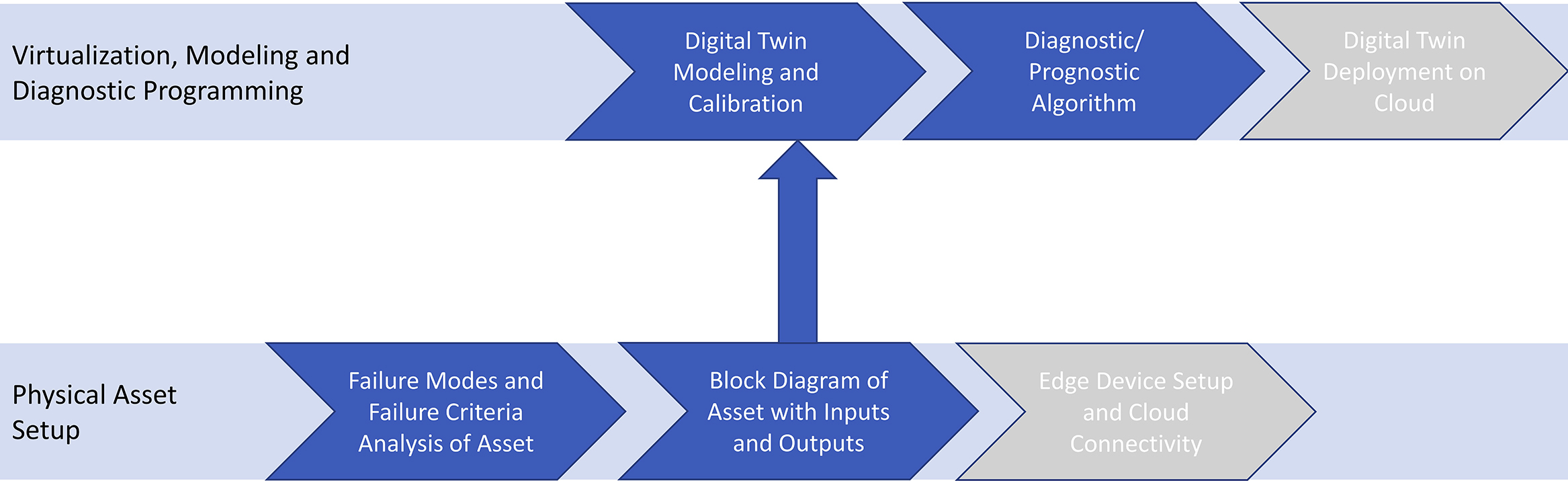
In this chapter, the focus will be on creating the digital twin model for the ball on plate. Fig. 4.1 shows the Off-BD steps that will be covered in this chapter. This includes failure modes for the asset, the block diagram, modeling of the digital twin, and a preliminary diagnostic algorithm. Edge device setup, connectivity, and deployment of the digital twin on the cloud are not covered.
All the codes used in the chapter can be downloaded for free from MATLAB File Exchange. Follow the link below and search for the ISBN or title of this book:
Alternatively, the reader can also download the material and other resources from the dedicated website or contact the authors for further help:
4.2. Ball on plate hardware
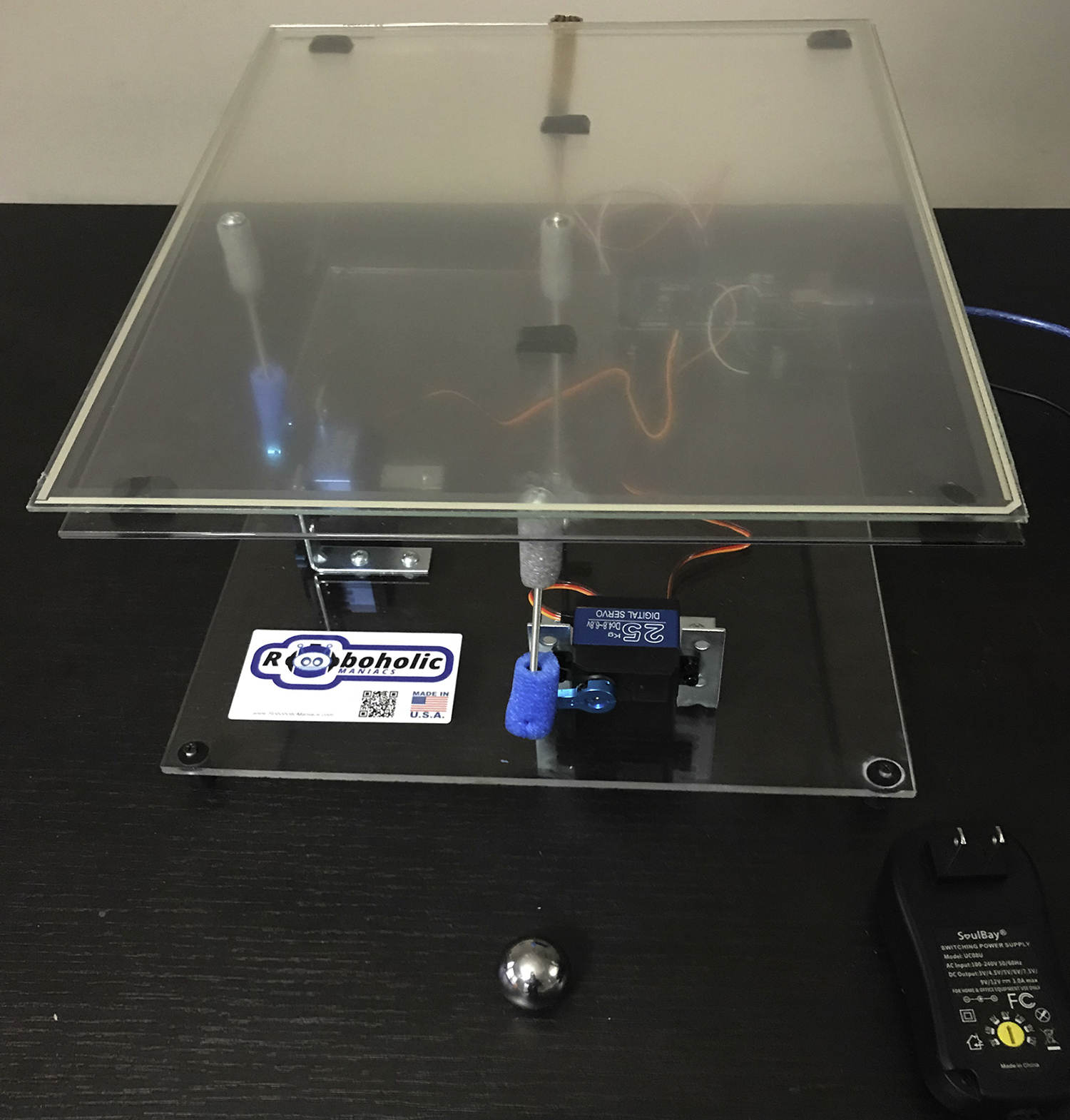
The ball on plate hardware was bought from RoboholicManiacs (www.roboholicmaniacs.com). The plate has two servo motors to control the x and y slope
of the plates. The plate is a touch screen of size 38
cm
×
24
cm and 2
cm thickness (Fig. 4.2). The ball is 1 inch in diameter and its mass is 51
g. The servo motors and the crankshaft mechanism are not modeled. Instead, the angle of the plate is an input to the SimscapeTM model.
4.3. Block diagram of the ball on plate system
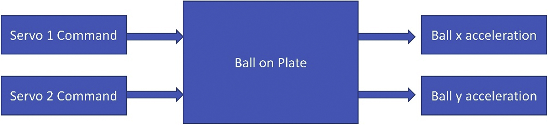
Ball on plate is a second-order multiinput and multioutput problem. The system has two inputs (in general there are two actuators) and two outputs (x and y position of the ball) (Fig. 4.3). The three main parts are the ball, the plate, and the actuation mechanism. The later can be actuated by servo motors or magnetic induction coils. The plate is generally constrained to rotate around the x and y axis (roll and pitch angles). The actuation mechanism modifies the two angles of the plate, which causes the
ball to roll due to gravity in the x and y directions. In many control problems, the objective is to maintain the ball at given coordinates despite external disturbances.
4.4. Failure modes and diagnostics concept for the ball on plate
In this chapter, we will focus on detecting failures that affect the acceleration of the ball. These failure modes include servo motor failure such as wiring issue, aging servo, or mechanical failure in the rotating mechanism. Failure could also include a stuck ball (due to dust or other obstacles). Lastly, failure in the sensing mechanism can also affect the ball acceleration.
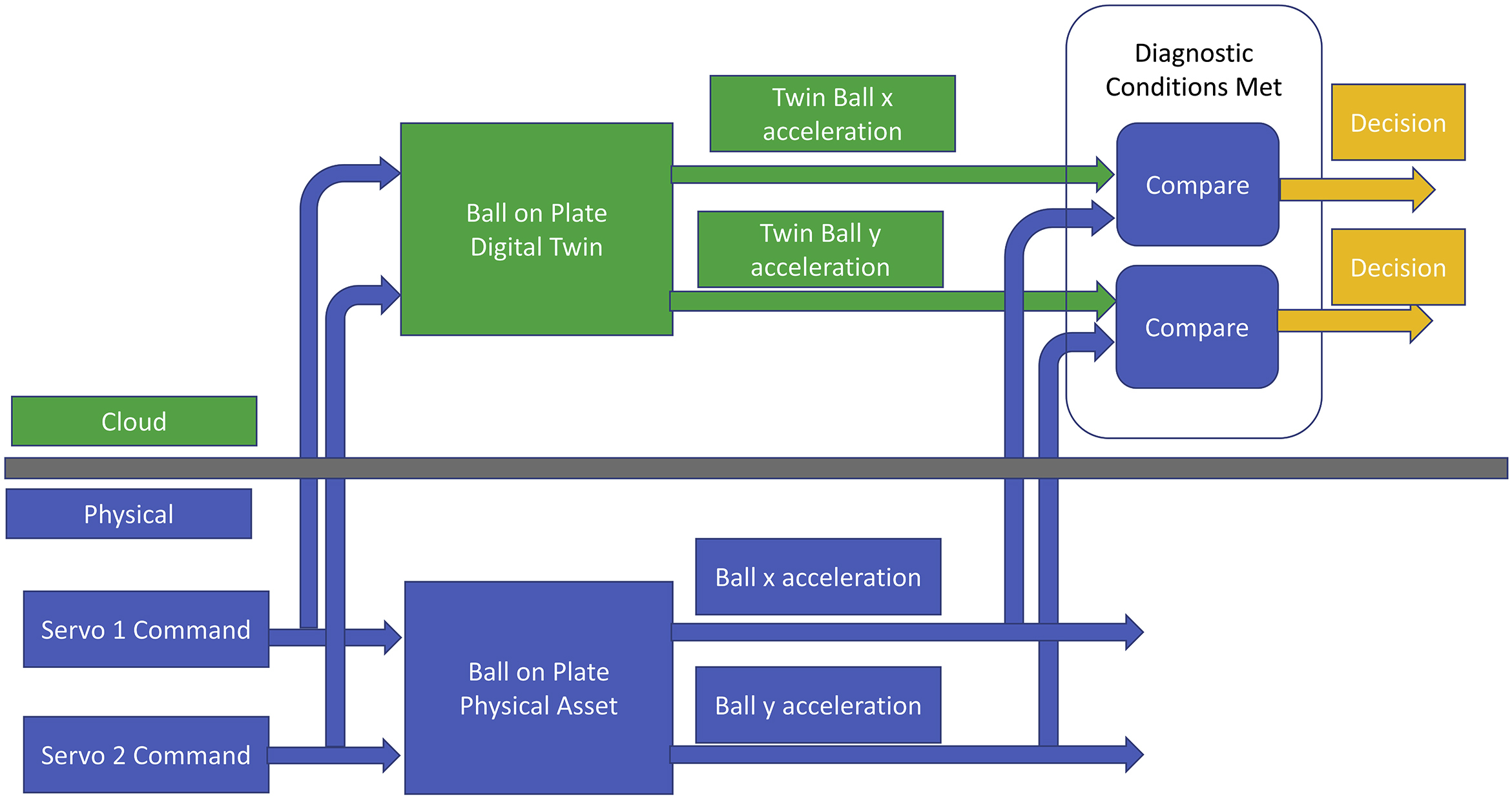
Regardless of the servo type or sensing mechanism, the process outlined to diagnose the system should still be applicable. The basic idea relies on acceleration measurement or estimation. If the acceleration of the physical asset deviates significantly from the acceleration of the digital twin, then a fault will be set. Usually the art of designing the diagnostic lies in implementing a logic that can look for the conditions where the deviations of the physical asset from the digital twin are magnified. This ensures a robust logic that can overcome uncertainties pertaining to modeling errors, slight aging of the hardware, uneven surface where the plate is place, and unmeasured disturbances (such as the air condition in the room blowing on the ball on plate setup). When implemented properly, implementing diagnostic enable conditions produces a detectable signal-to-noise ratio.
We will enable the diagnostic when either the servo command or the acceleration of the ball is big. For few samples of time, the digital twin and physical asset average accelerations will be compared. If the difference is bigger than a threshold, then a fault will be set. Fig. 4.4 shows the diagnostic process.
4.5. Simscape model for the ball on plate
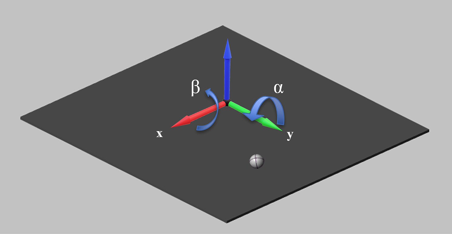
To create the digital twin, we will use Simscape MultibodyTM (formerly known as SimMechanicsTM). The inputs to the model will be the angles of the plate while the outputs will be x and y position of the ball. Furthermore, we will integrate the model with two PID controllers. Using Mechanics Explorer, we will watch and record the transient response of the ball. The simulation will be recorded as a video for playback and demo purposes. Fig. 4.5 shows the Cartesian coordinate as well as the rotation angles of the plate.
The challenge in modeling this application using SimscapeTM is that unlike most of components in Simscape Multibody, ball and the plate are not connected by a joint, a belt, or are constrained to be in contact. This means the custom equations between the ball and the plate have to be developed and solved explicitly in Simulink or in user-defined subsystem and not by SimscapeTM solver.
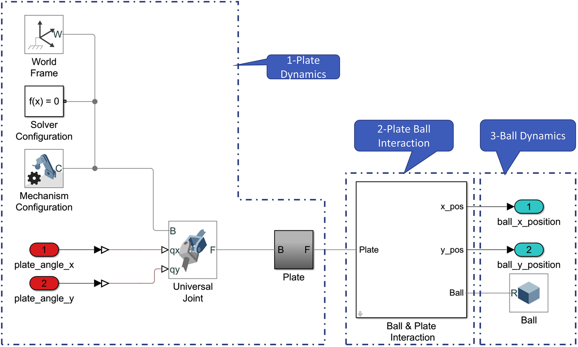
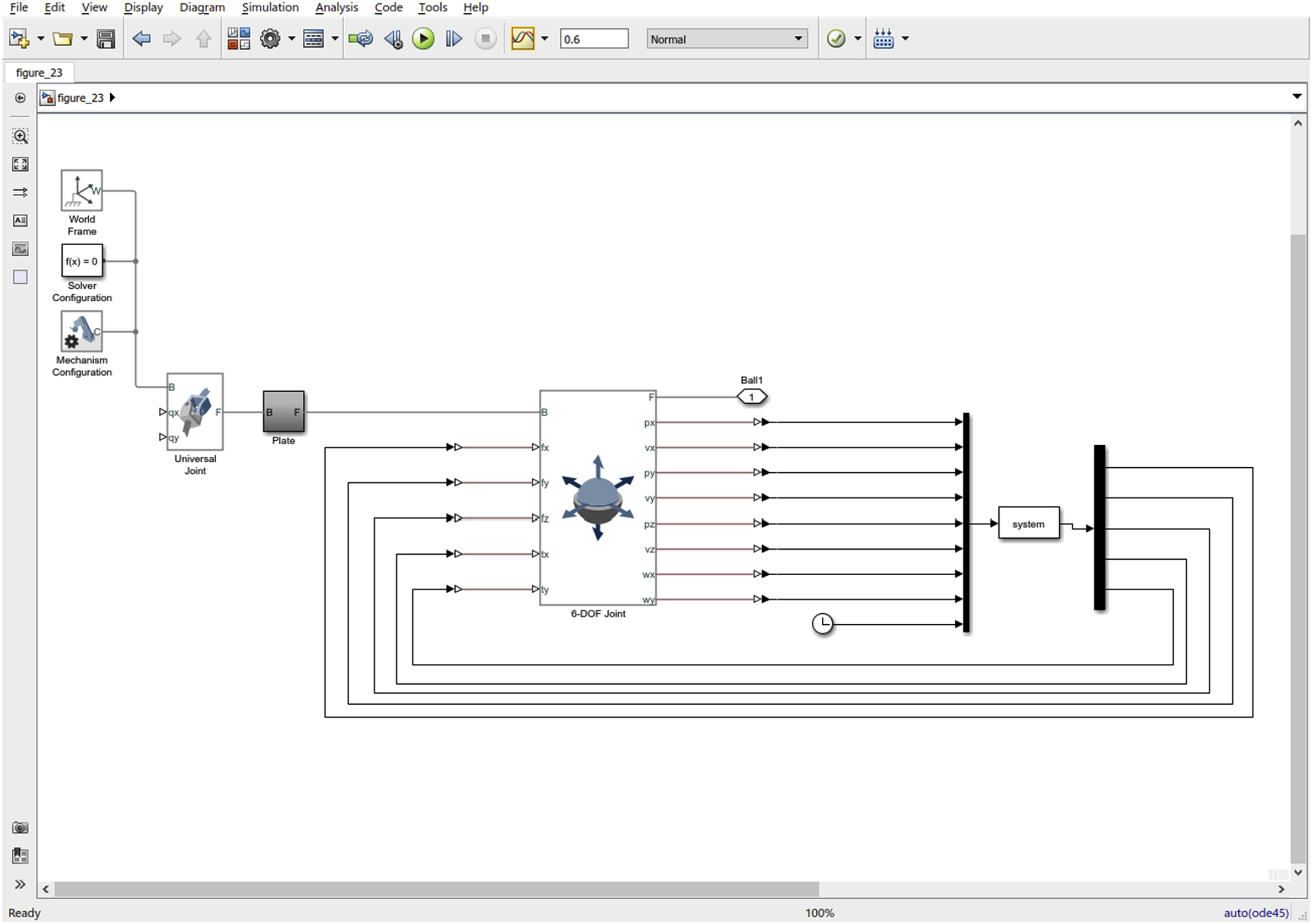
The final model is shown in Fig. 4.6. The main components are
Like we mentioned in previous chapters, unlike Simulink®, there is no directionality of signal flow in SimscapeTM. Summarizing the basic idea behind Fig. 4.6, we have a world frame. The world frame serves as the universal frame. It is connected to 2 degree-of-freedom (DOF) joint. This joint allows the user to set the two angles for the plate. The universal joint is connected to the solid shape block of the plate. It contains the mass, inertia, geometry, and graphics of the plate. The plate is connected to the ball and plate interaction block. The block has the 6 DOF joint for the ball as well as the s-function that calculates the forces between the ball and plate. Finally, the ball
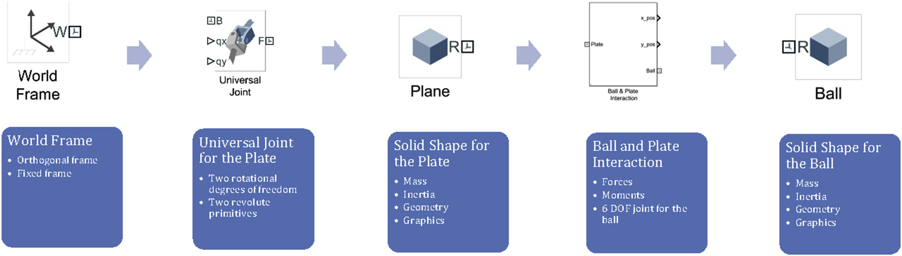
geometry is connected as a follower frame to the 6-DOF joint for ball. Fig. 4.7 shows the main elements of the ball on plate model.
Below are the detailed steps to building the Simscape® model:
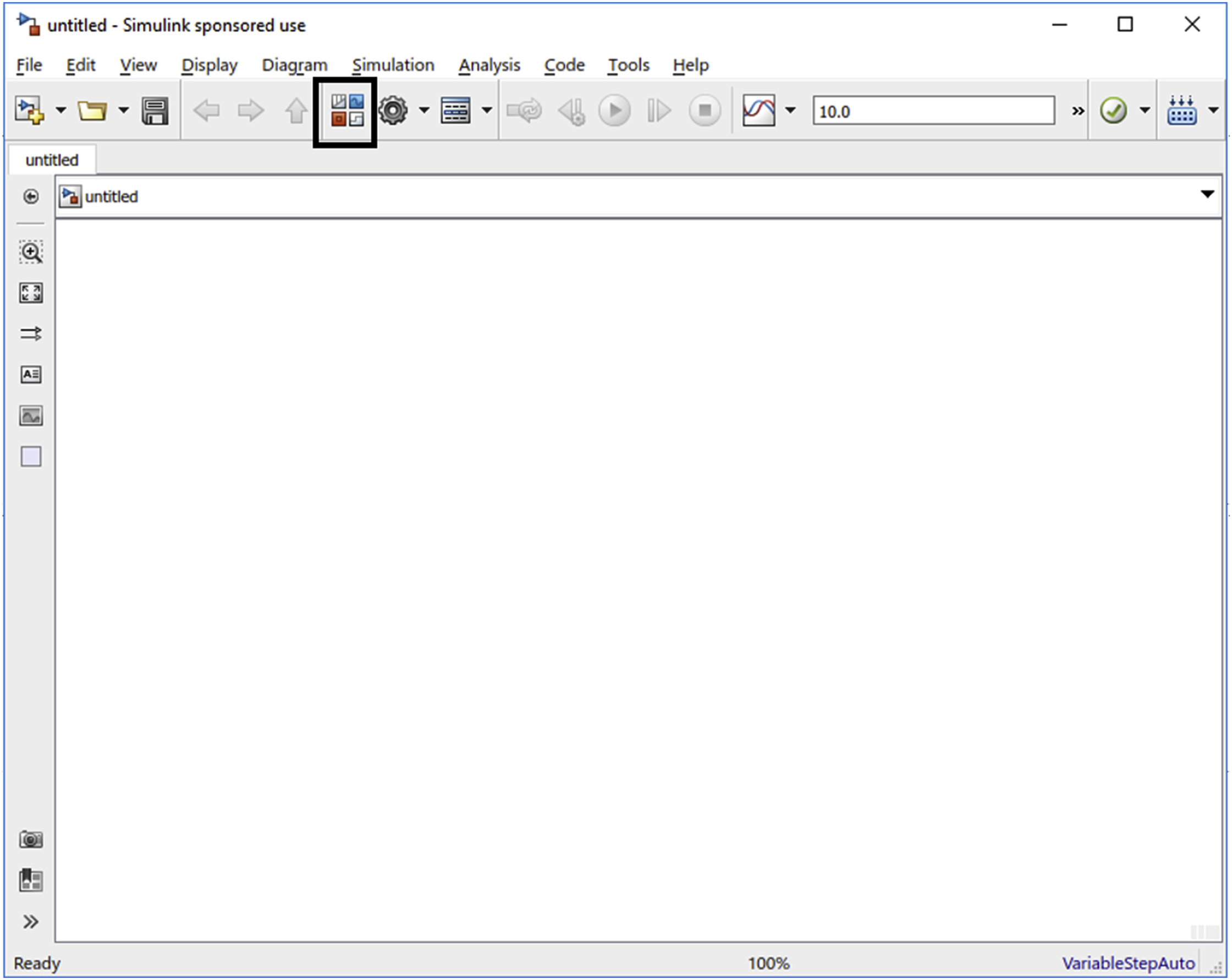
- Step 1: Create a new Simulink® model.
- Step 2: Press the Simulink® Library Browser (Fig. 4.8).
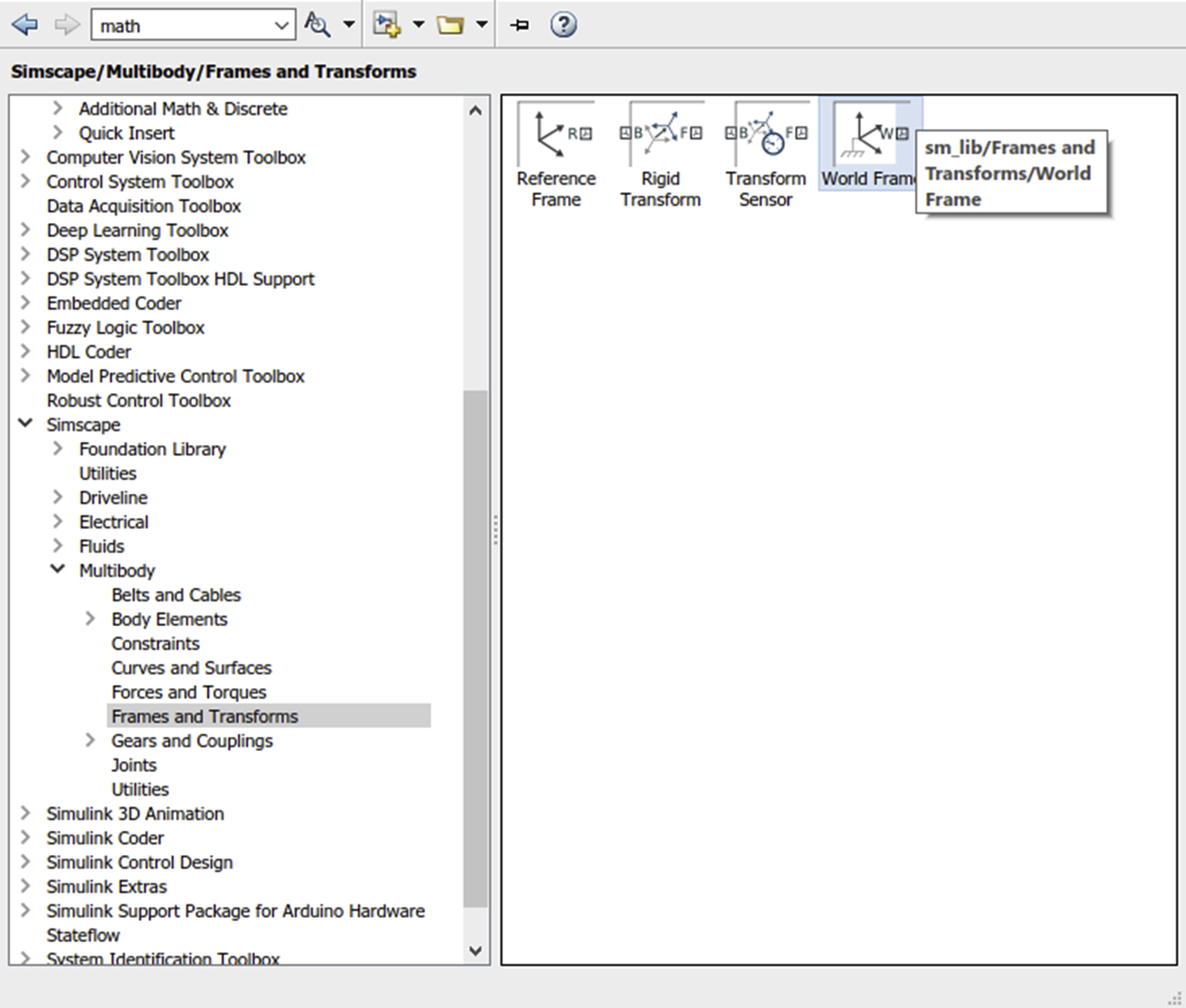
- Step 3: Navigate to Simscape> Multibody Library>Frames and Transforms and add World Frame block to the model (Fig. 4.9).
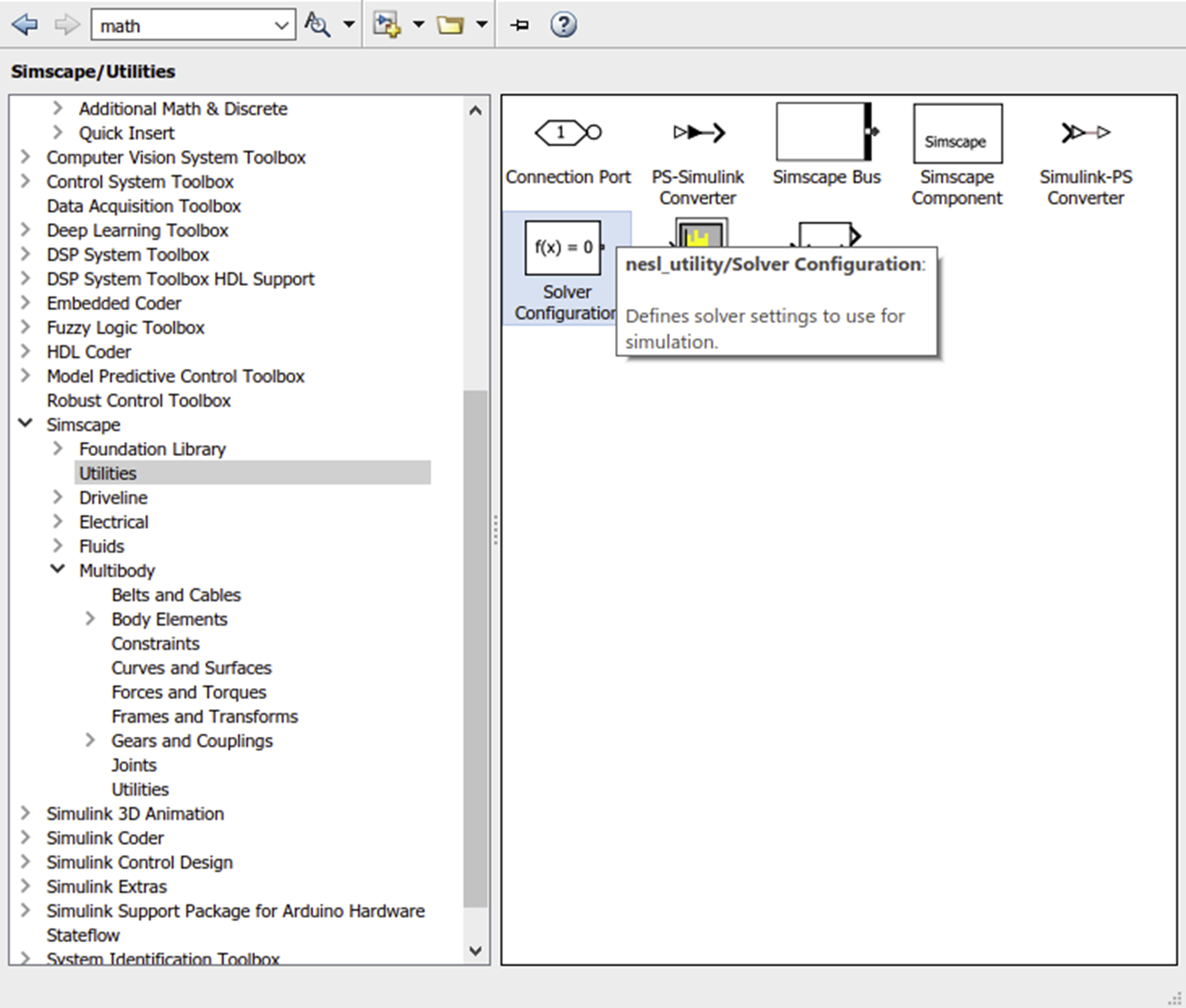
- Step 4: Go back to Simscape> Utilities and add Solver Configuration block (Fig. 4.10).
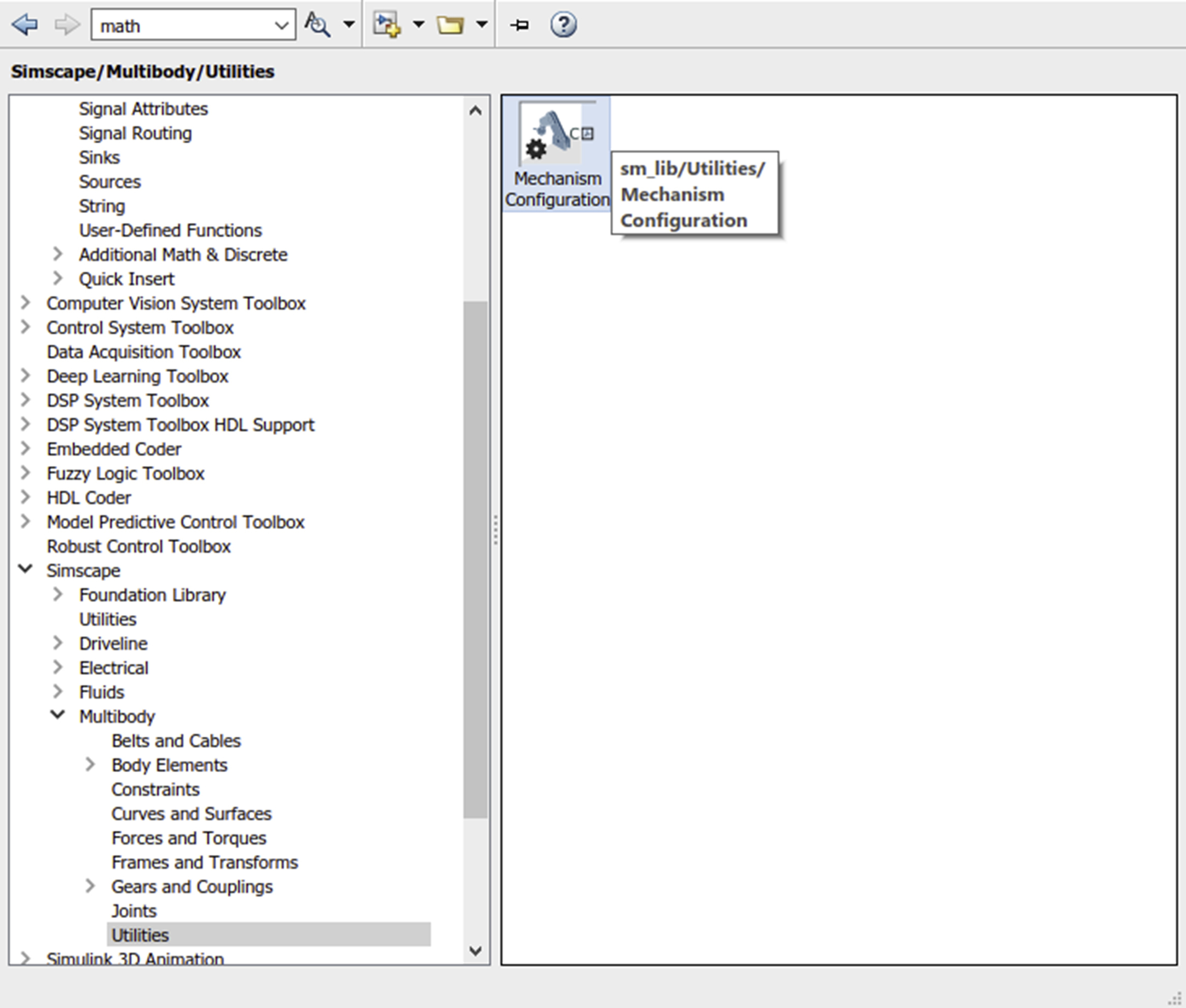
- Step 5: Go to Multibody>Utilities and add Mechanism Configuration block (Fig. 4.11).
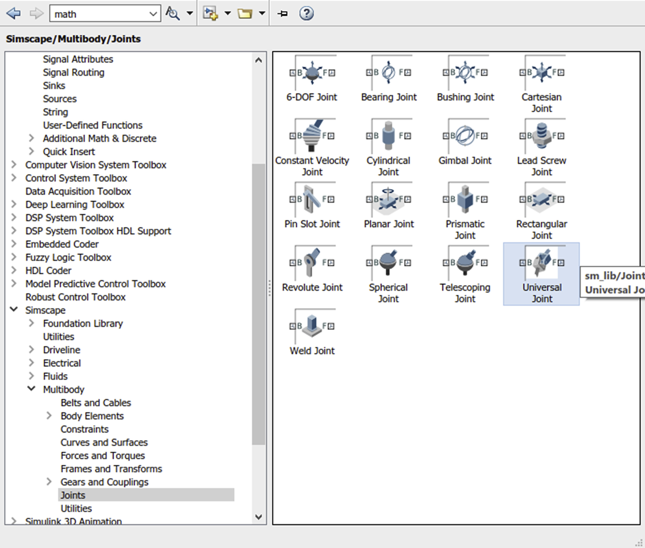
- Step 9: Go to Multibody>Joints and add Universal Joint block to the model (Fig. 4.12).
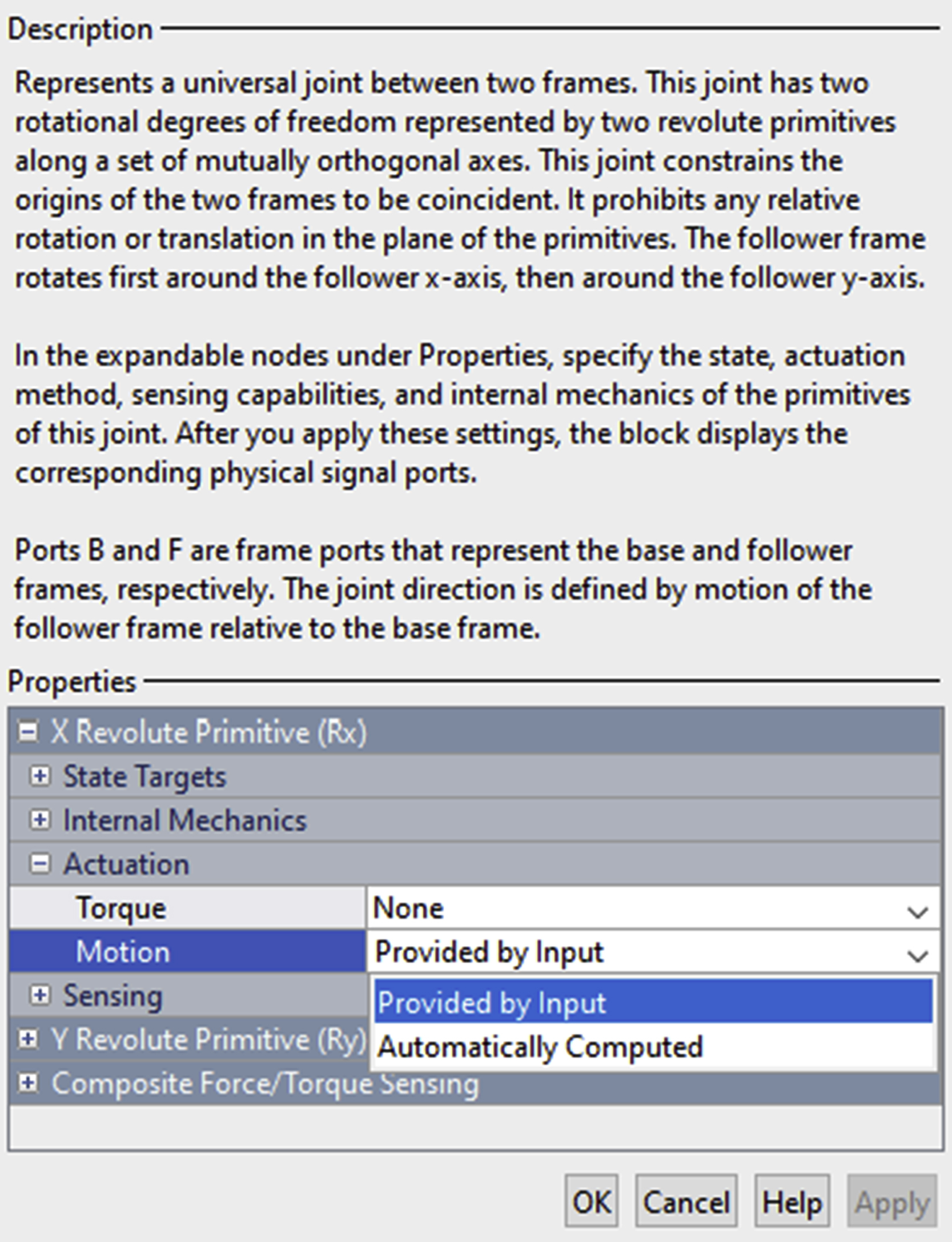
- Step 10: To force the plate to have the angles as input, double click the Universal Joint and change the settings Actuation>Motion>Provided by input for both the X Revolute Primitive (Rx) and Y Revolute Primitive (Ry) (Fig. 4.13). Note that these angles need to be provided in radians.
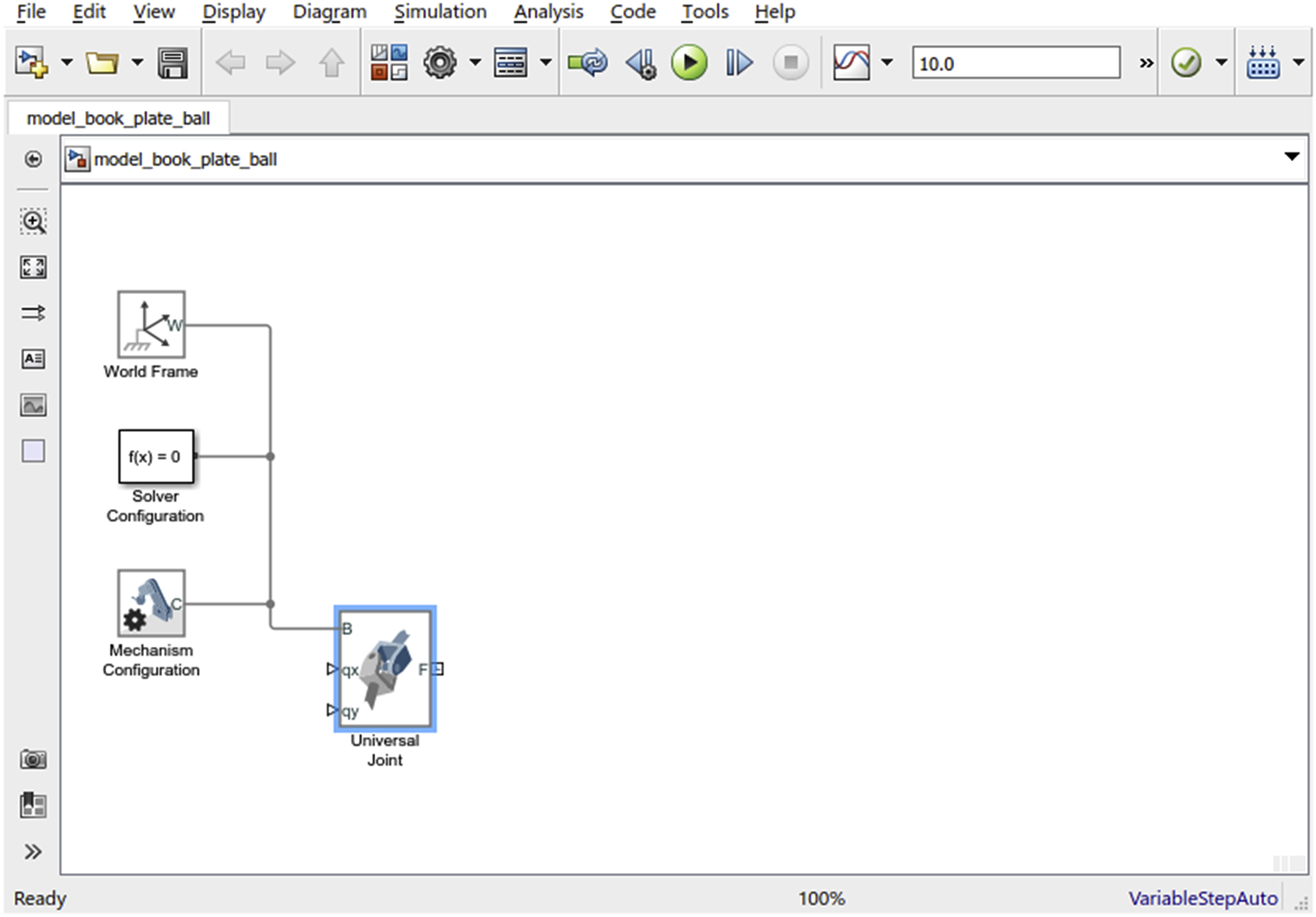
- Step 10: Connect all the previously mentioned blocks to the Universal Joints (Fig. 4.14). To do so, connect one block to the Universal Joint and connect the rest to the connecting line. Connecting Simscape blocks is a bit different than connecting Simulink blocks.
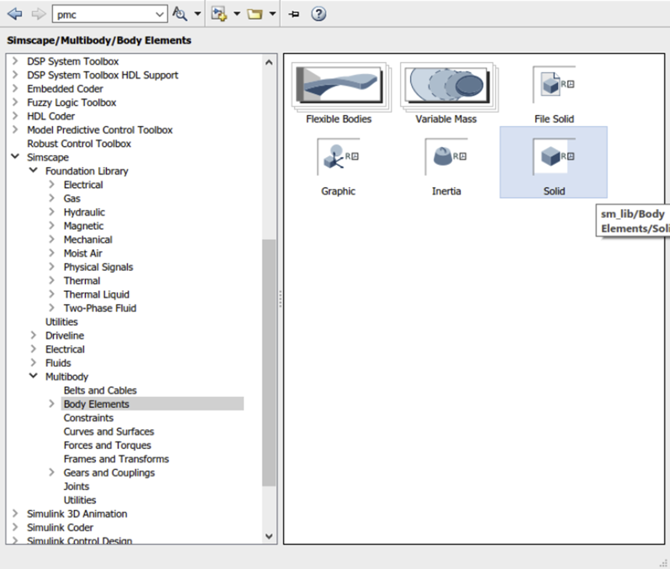
- Step 11: To create the physical object representing the plate, add the Solid block from the Simscape>Multibody Library> Body Elements Library (Fig. 4.15).
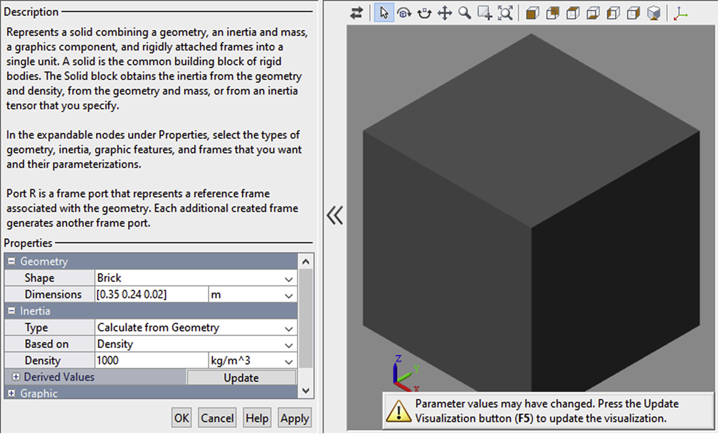
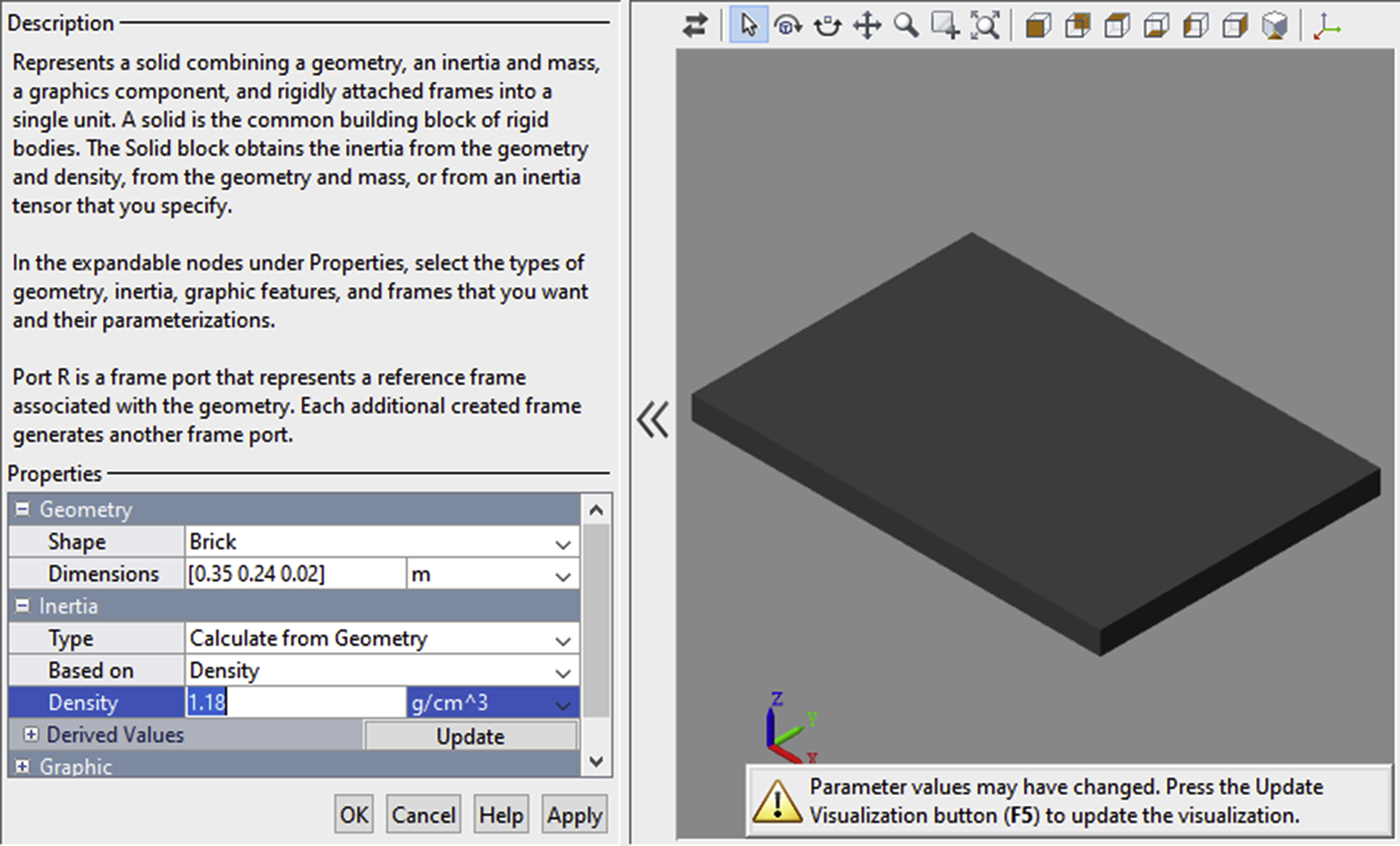
- Step 12: Double clock the Solid block and change the dimensions of the plate to [0.38, 0.25, 0.02] m, which represent the dimensions of the plate (Fig. 4.16).
- Step 14: Change the density to 1.18 g/cm³ since the plate is plexiglass (Fig. 4.17).
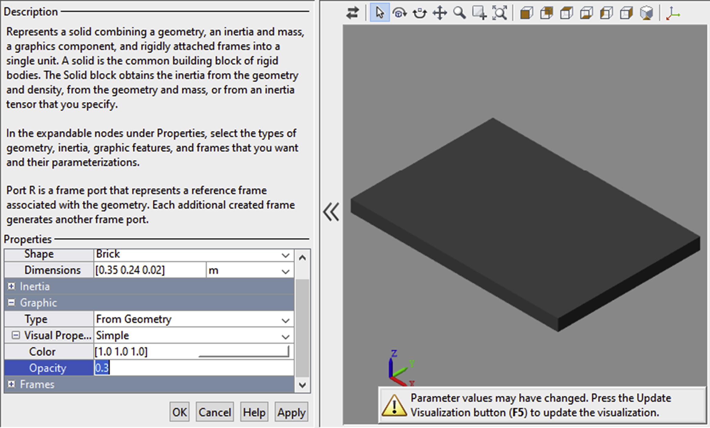
- Step 15: Change the Color and Opacity to your desired values (Fig. 4.18).
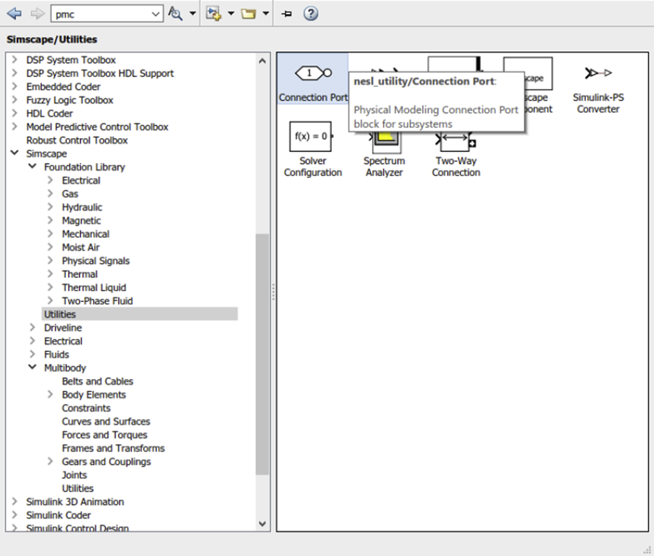
- Step 16: Add two connection ports to the model from the Simscape>Utilities (Fig. 4.19).
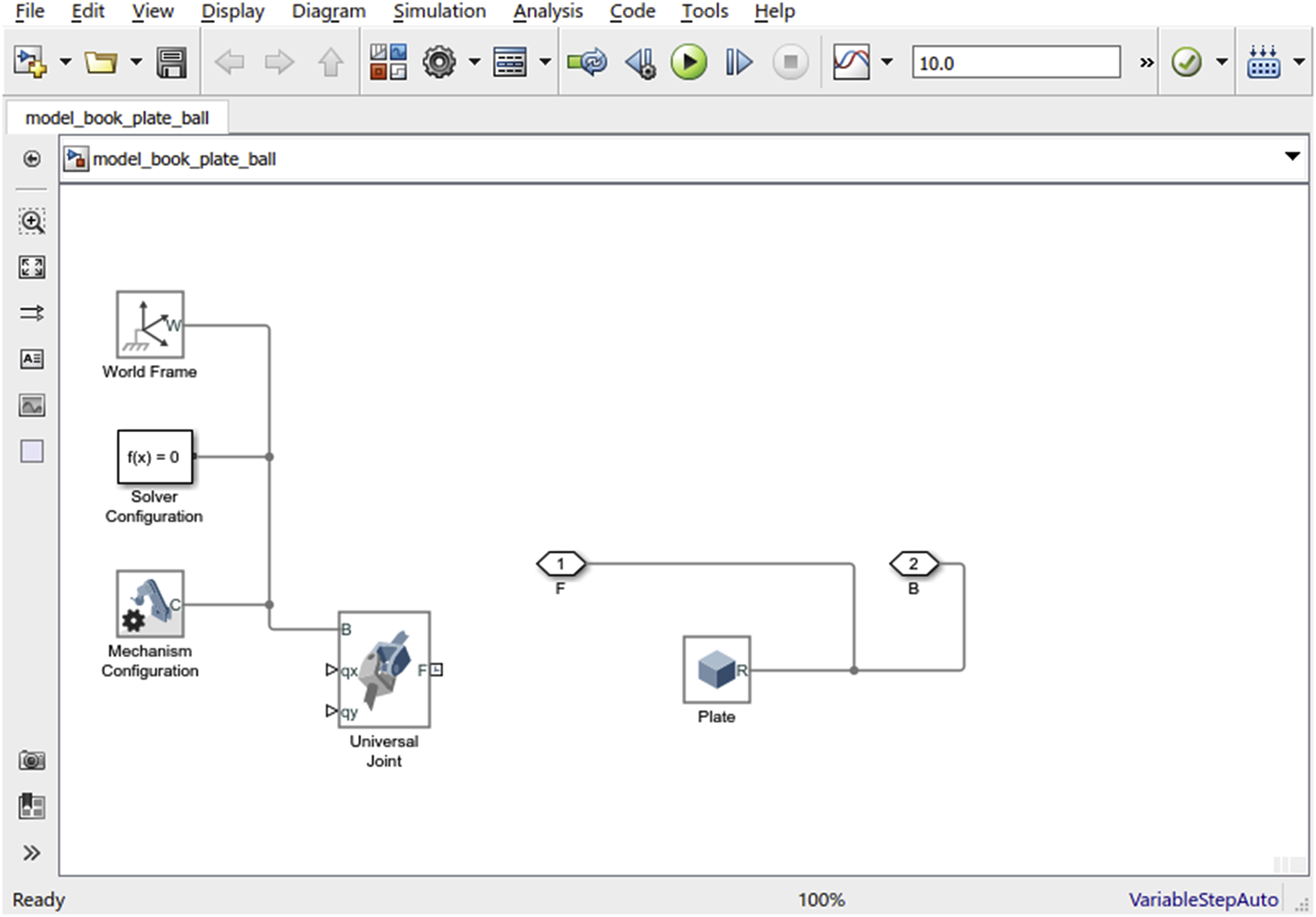
- Step 17: Rename the ports F and B, respectively, by clicking once on the block and then editing the name underneath the block. Do the same for the Solid and rename it Plate (Fig. 4.20).
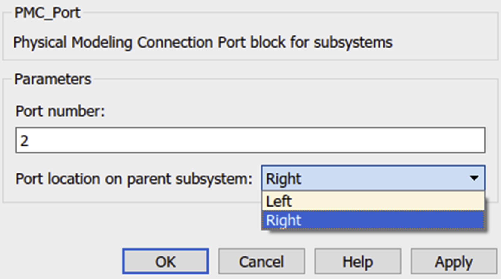
- Step 18: For better display when we create a subsystem for the components, double click the connection port named B, and change the port location to the right (Fig. 4.21).
- Step 19: Connect the B connection port to the Solid and then connect F connection port to the connection line.
- Step 20: Select F and B connection ports along with the Plate and create a subsystem (Fig. 4.22).
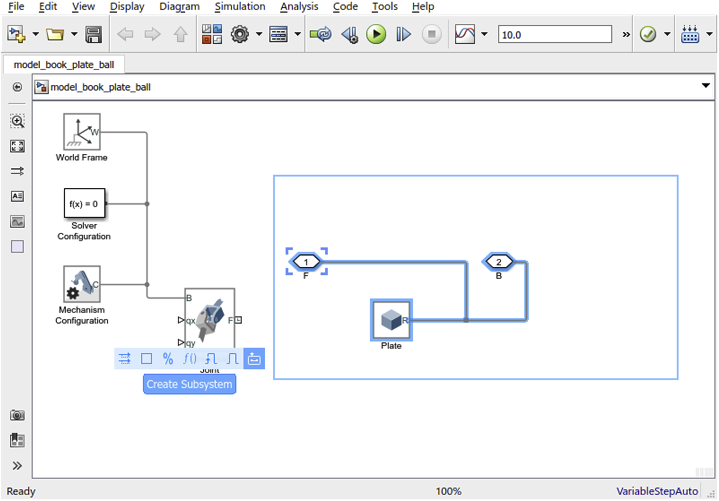
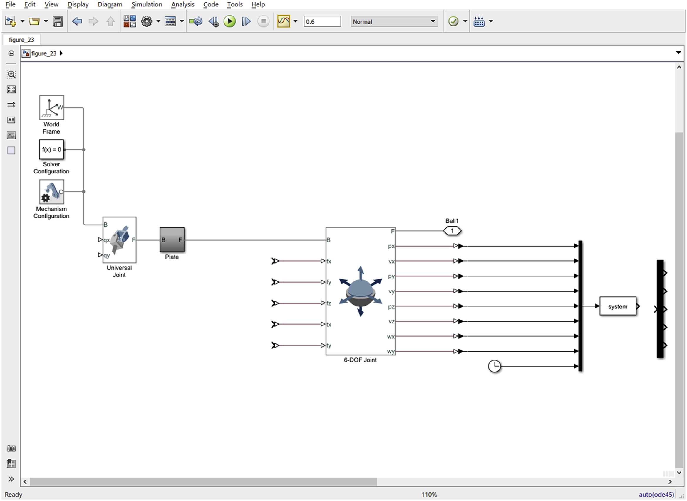
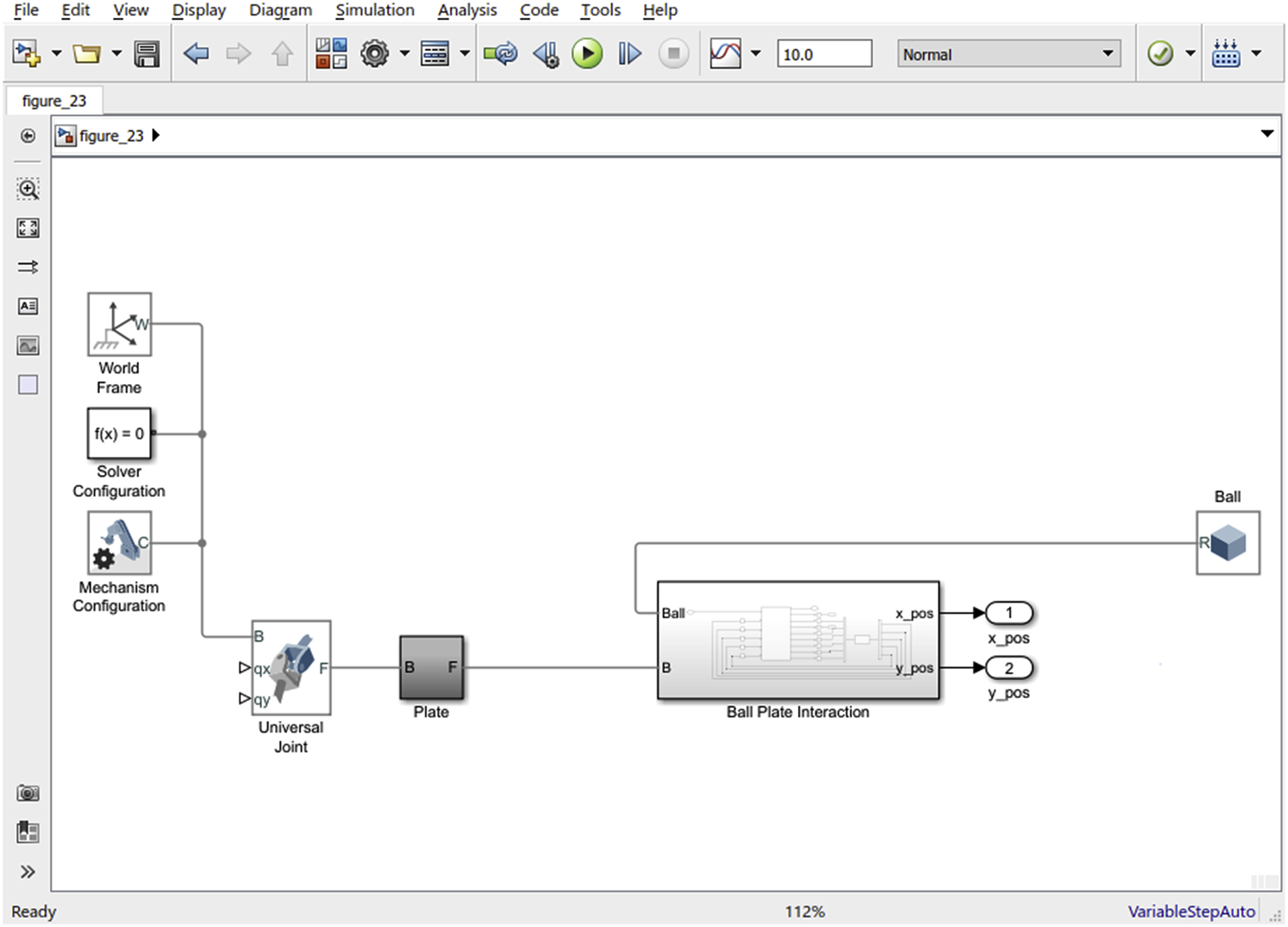
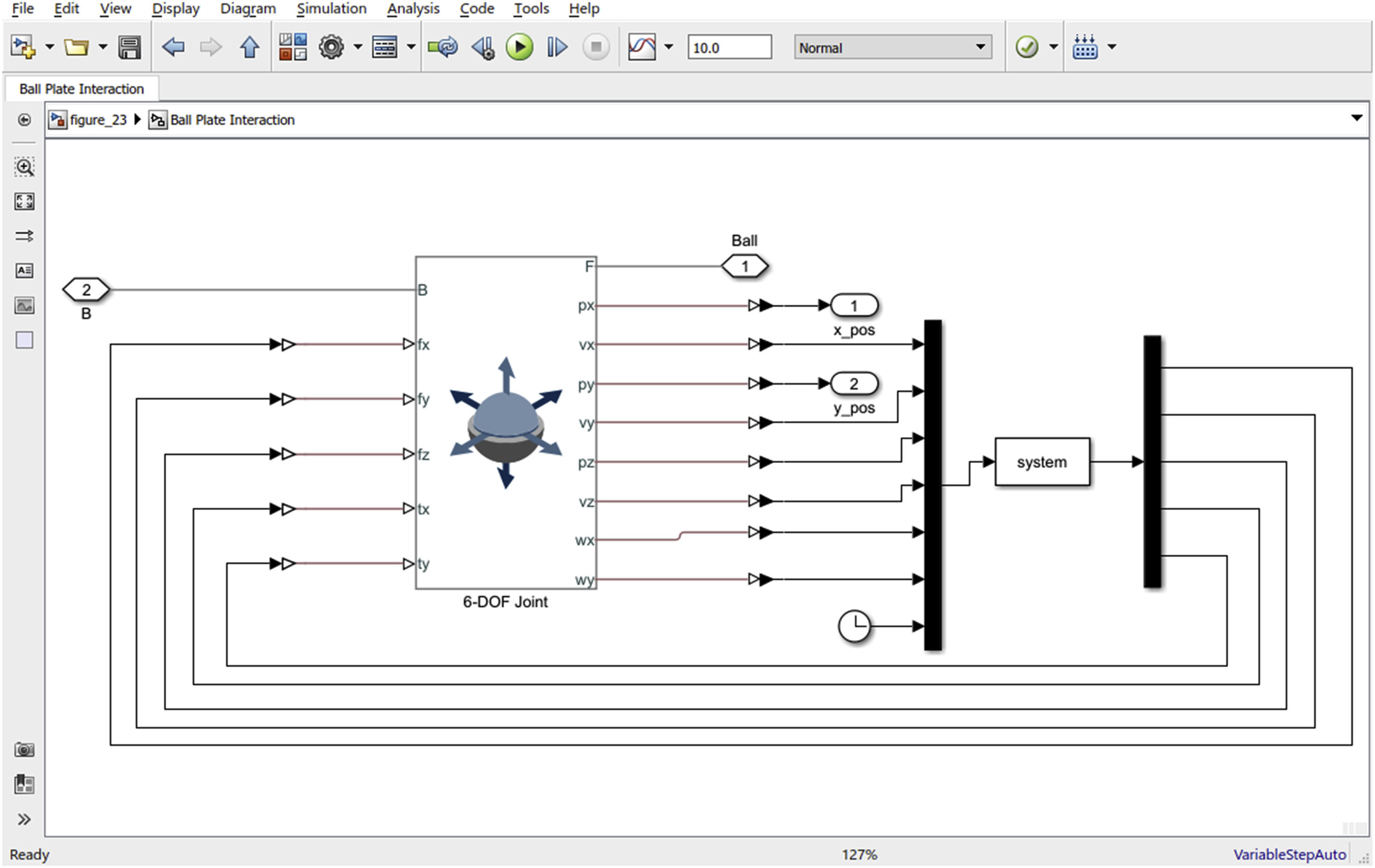
- Step 21: Rename the subsystem Plate and remove the input and output ports named F and B. The model is shown in Fig. 4.23.
- Step 22: Connect the Universal Joint to the Plate subsystem. Note that the order of the blocks and creating the subsystem are for better presentation of the model. Both F and B connection ports are identical except for the name and location of the block.
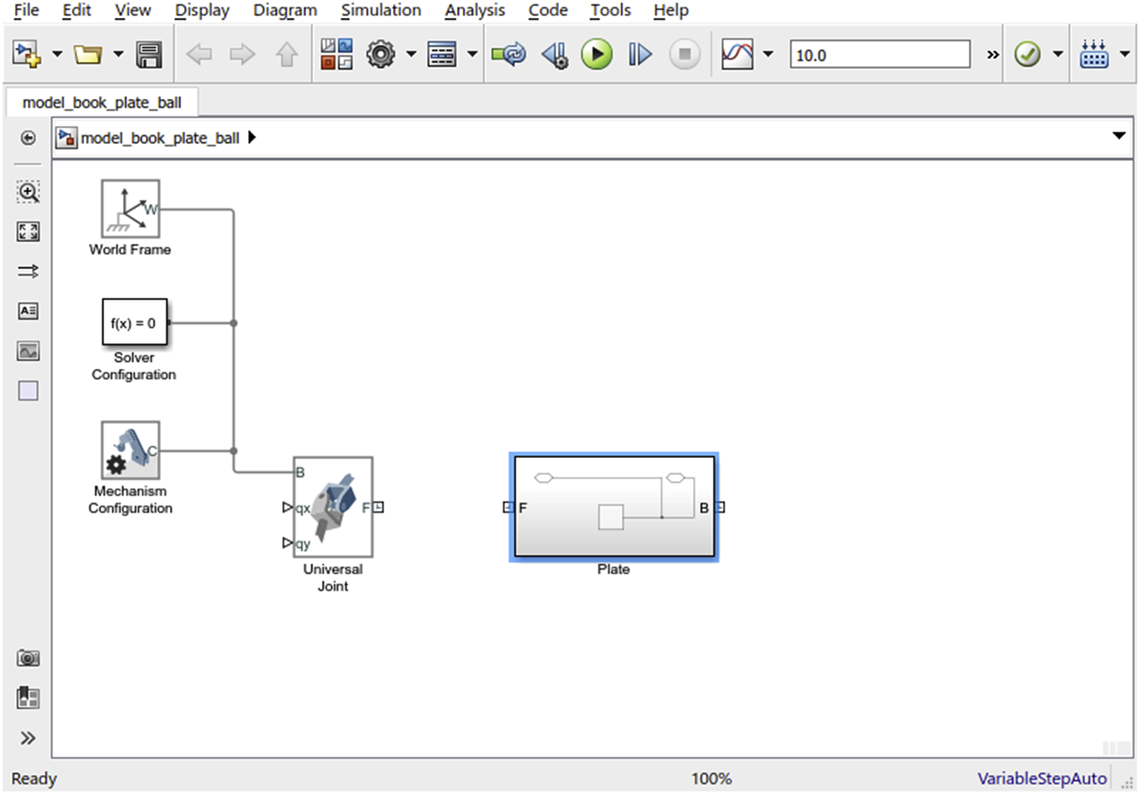
- Step 23: Go to Simscape>Multibody>Joints and add 6-DOF Joint to the model (Fig. 4.24). This will be used as the reference frame for the ball. The ball exhibits both translation and rotation.
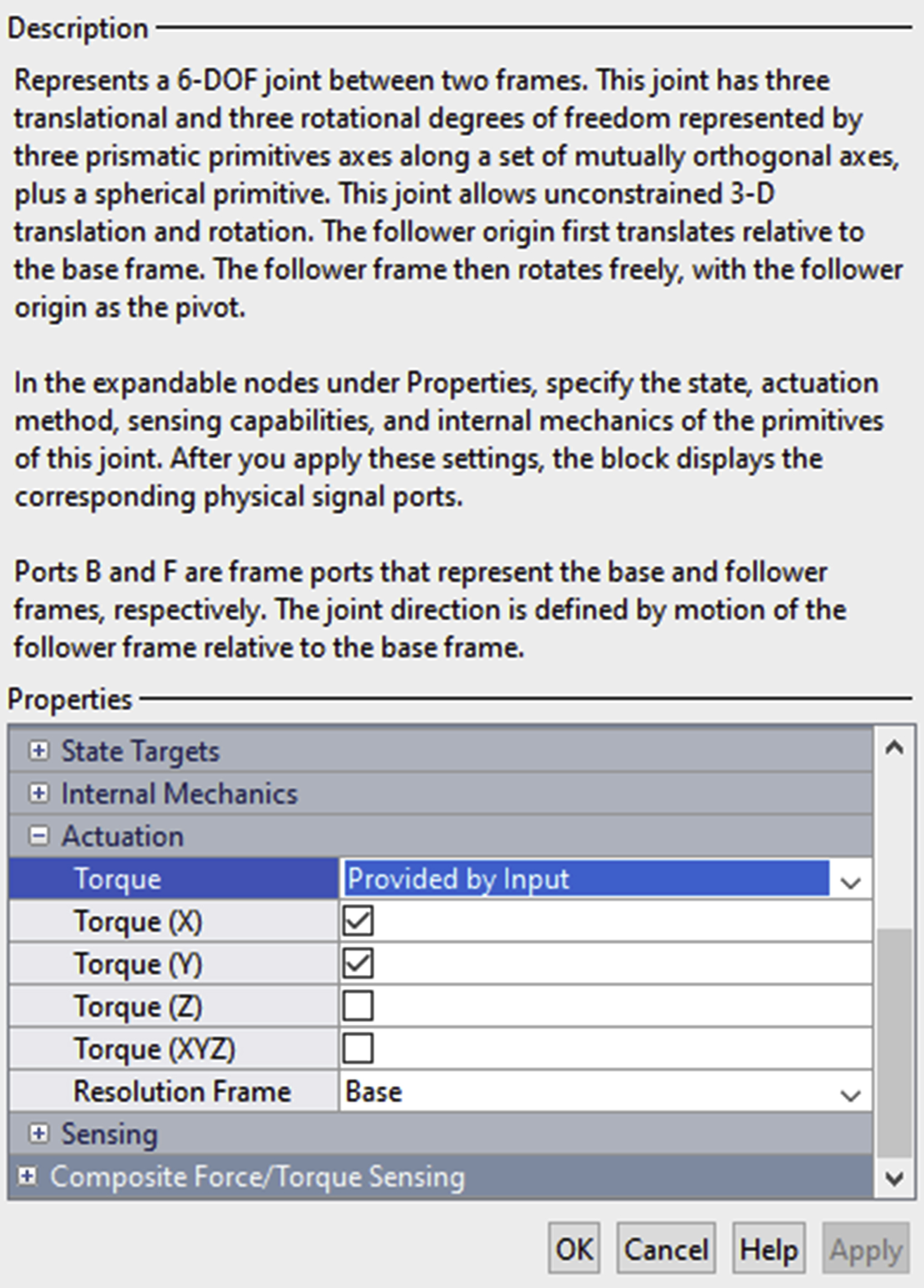
- Step 24: The plate exerts friction forces (fx and fy) on the ball in the x and y directions. Additionally, the plate exerts a normal component force, fz, that constrains the ball from falling through the plate. Finally, the friction forces (fx and fy) form torques (tx and ty) on the sphere. All these forces and torques need to be setup as inputs to the 6-DOF Joint. Fig. 4.25 shows how to setup the forces fx as an input to the joint. Similarly, fy and fz can be setup. Fig. 4.26 shows how to setup tx and ty.
- Step 25: Stretch the 6-DOF Joint block to a bigger size for a better visibility of the inputs.
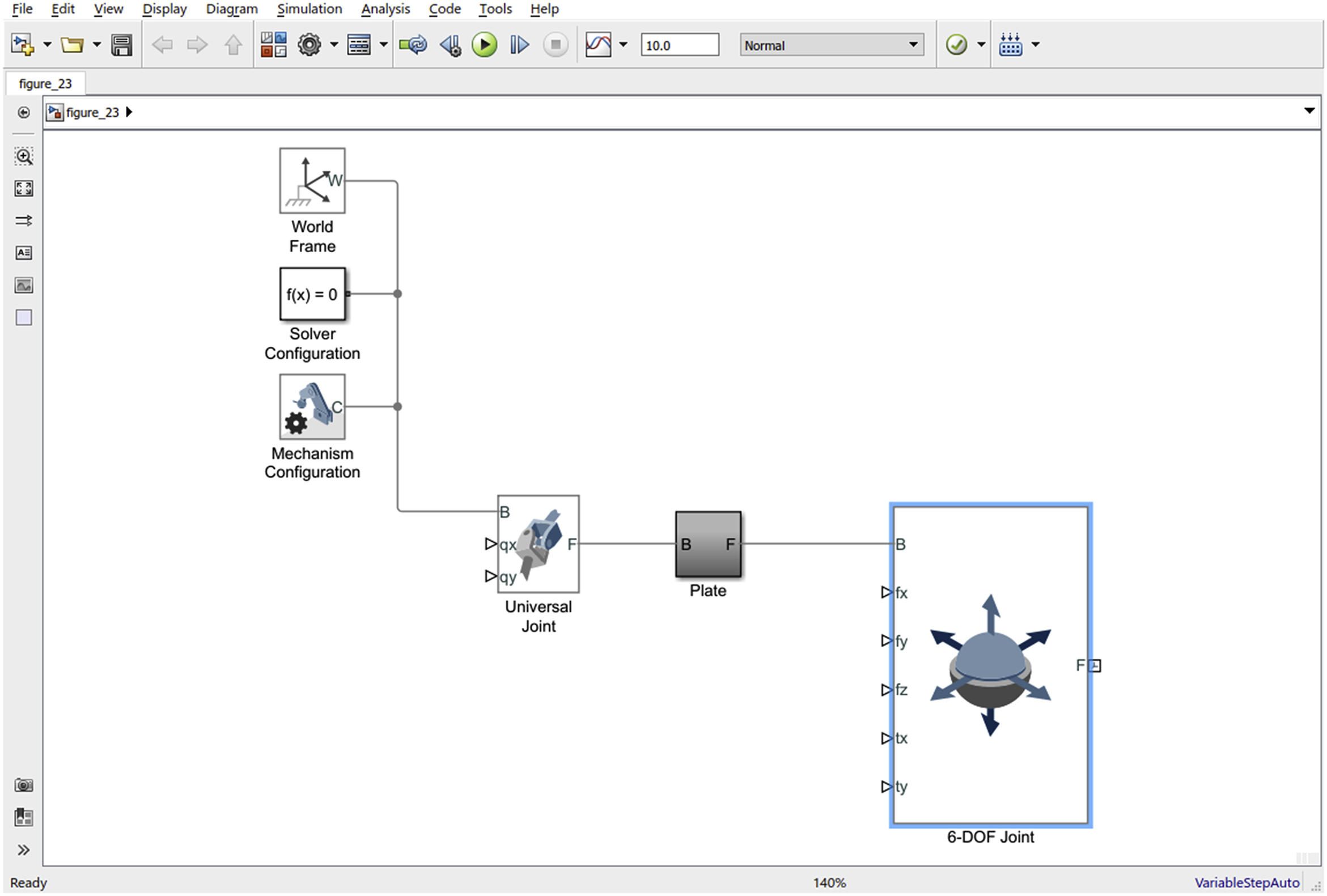
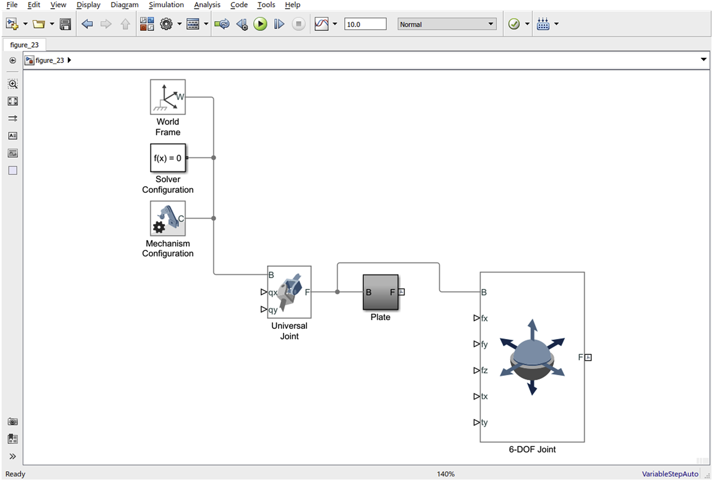
- Step 26: Connect the F port of the Plate block to the B port of 6-DOF Joint (Fig. 4.27). Alternatively, we could have connected the Universal Joint to the 6-DOF Joint (Fig. 4.28). The objective is to make the 6-DOF Joint a follower frame relative to the Universal Joint.
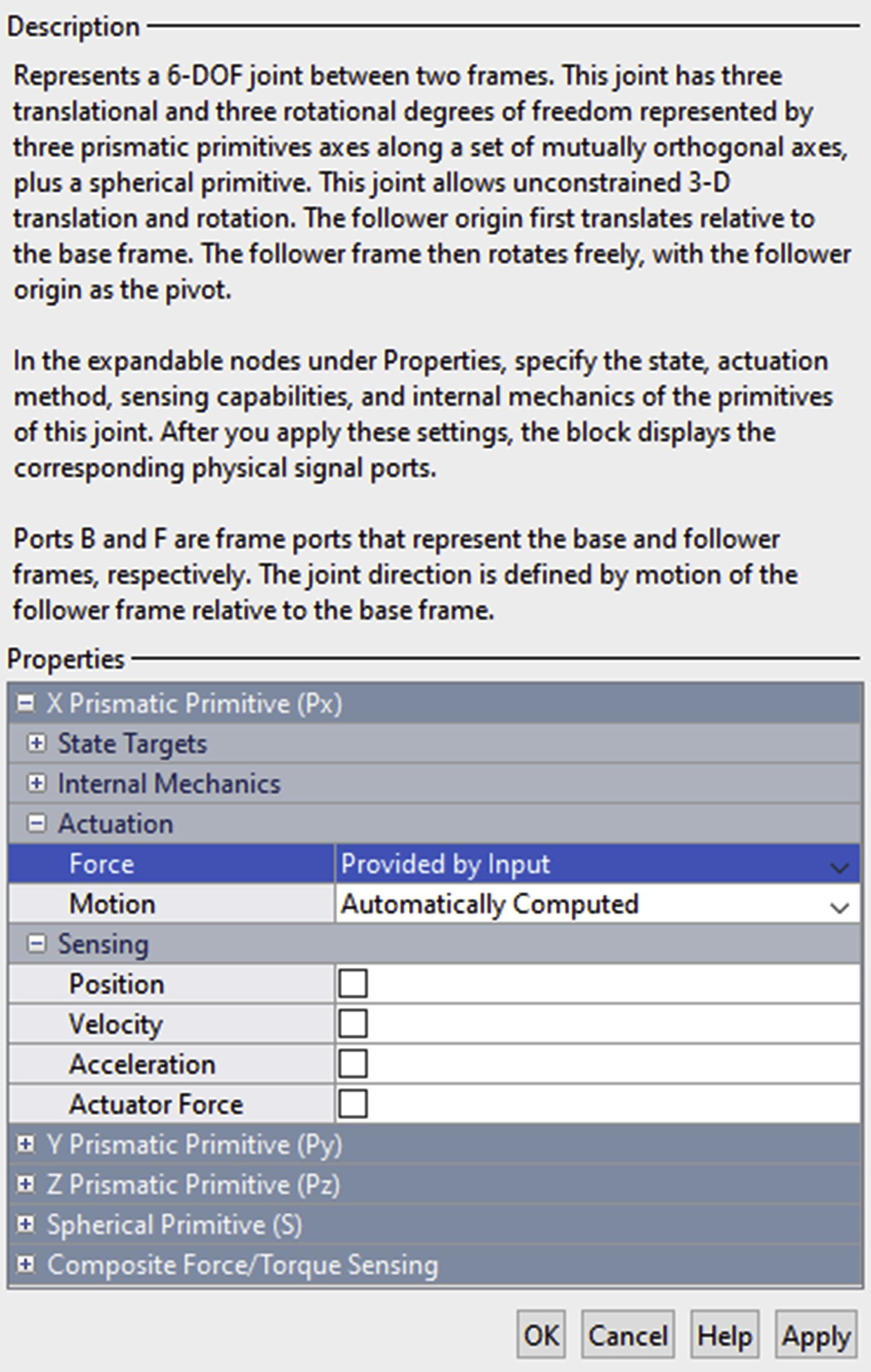
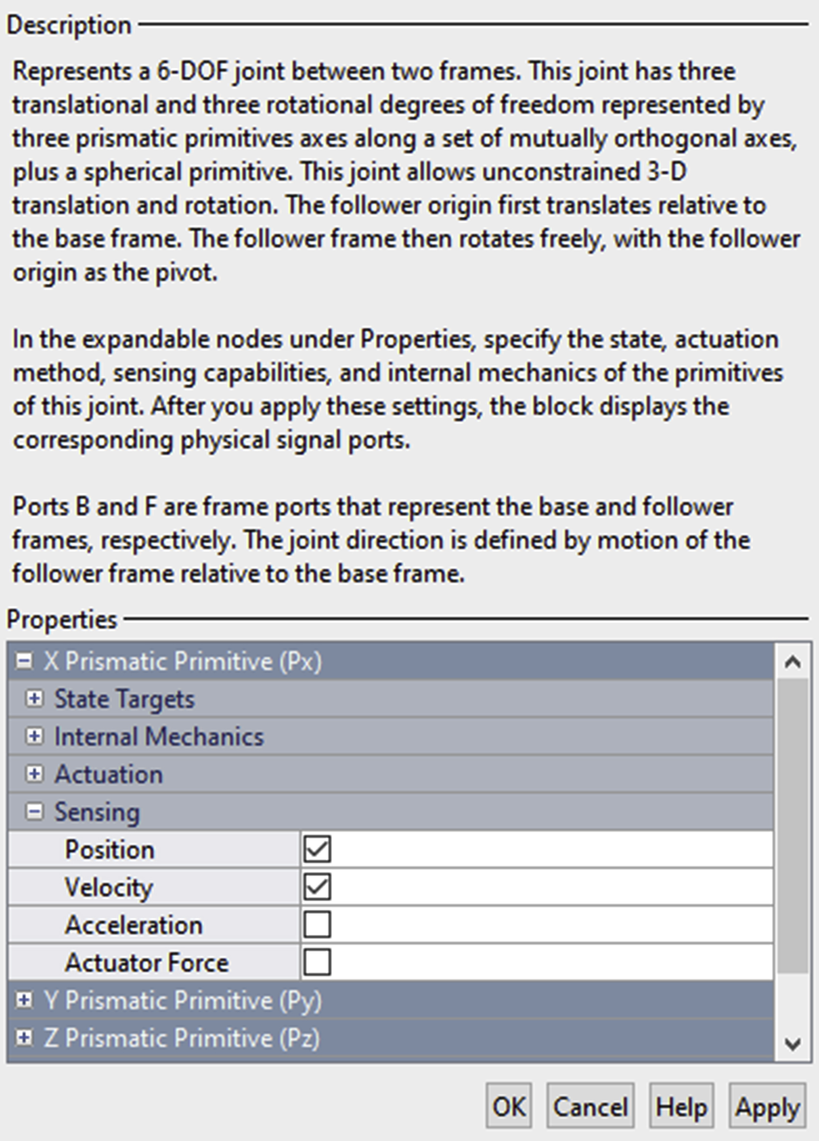
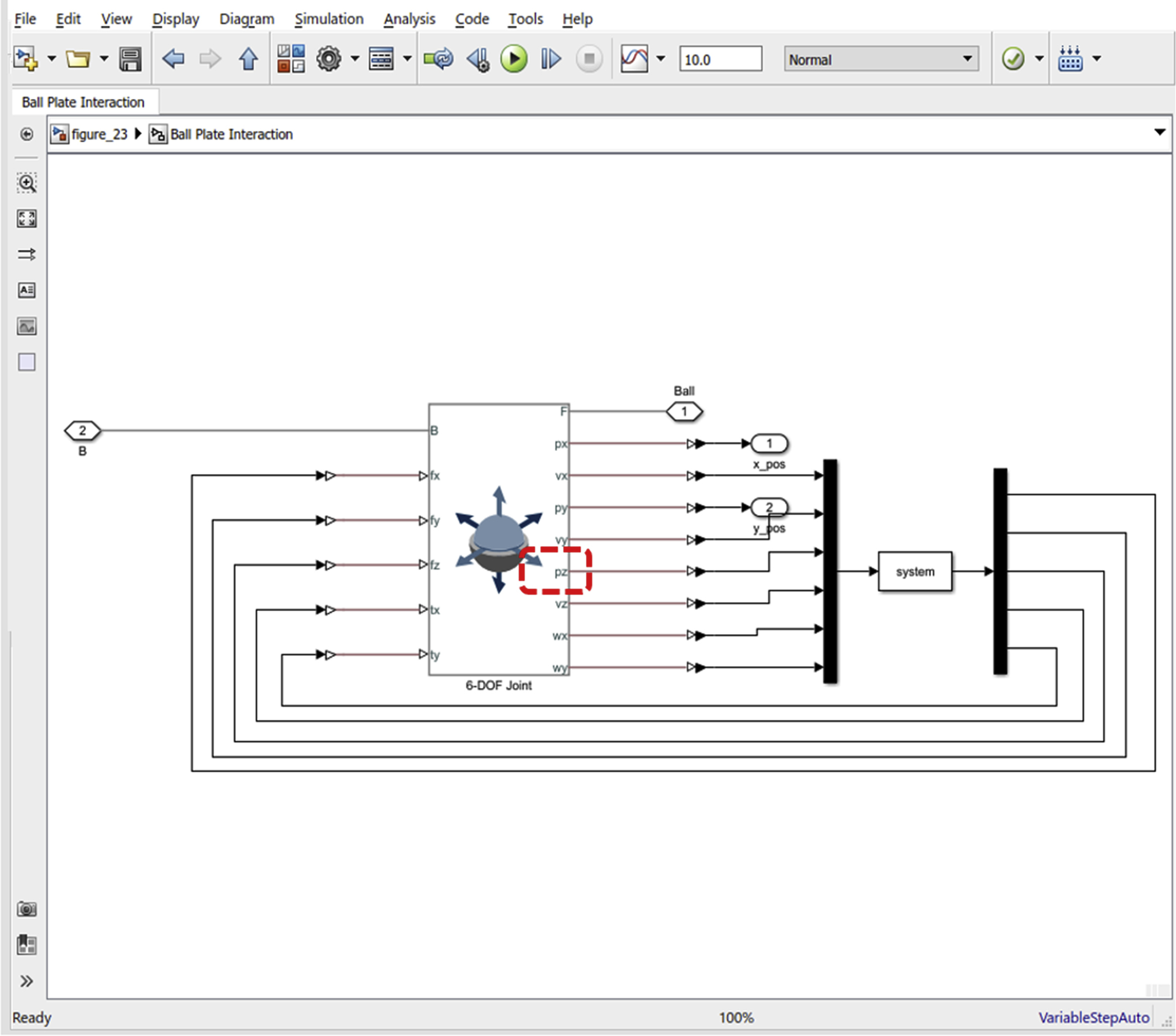
- Step 27: We need a set of outputs (measurements) from the 6-DOF Joint to allow us to compute the ball and plate interaction. Double click the 6-DOF Joint block, and tick the Position and Velocity boxes for the X Prismatic Primitive (Px), Y Prismatic Primitive (Py), and Z Prismatic Primitive (Pz) (Fig. 4.29). For rotational measurements, tick the Velocity (X) and Velocity (Y) for the Spherical Primitive (S). These represent the rotational speed around the X and Y axis.
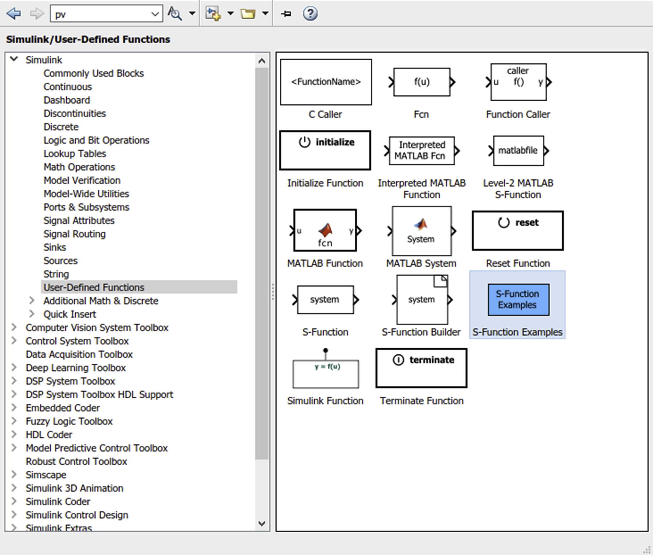
- Step 28: From Simulink>User-Defined Functions add an S-Function. In this block, we will embed the c script, ballplateforces.c, that will include the calculation of the friction forces and moments of the plate on the ball in addition to the support forces in the z-direction. The c script will be discussed in the next section.
- Step 29: From Simulink> Commonly Used Blocks, add a Mux and Demux blocks.
- Step 30: The inputs for the c script, ballplateforces.c, are px, vx, py, vy, pz, vz, wx, and wy. Additionally, simulation time will be an input. Change the number of Mux inputs to 9.
- Step 31: The outputs for the c script, ballplateforces.c, are fx, fy, fz, tx, and ty. Change the number of Demux outputs to 5.
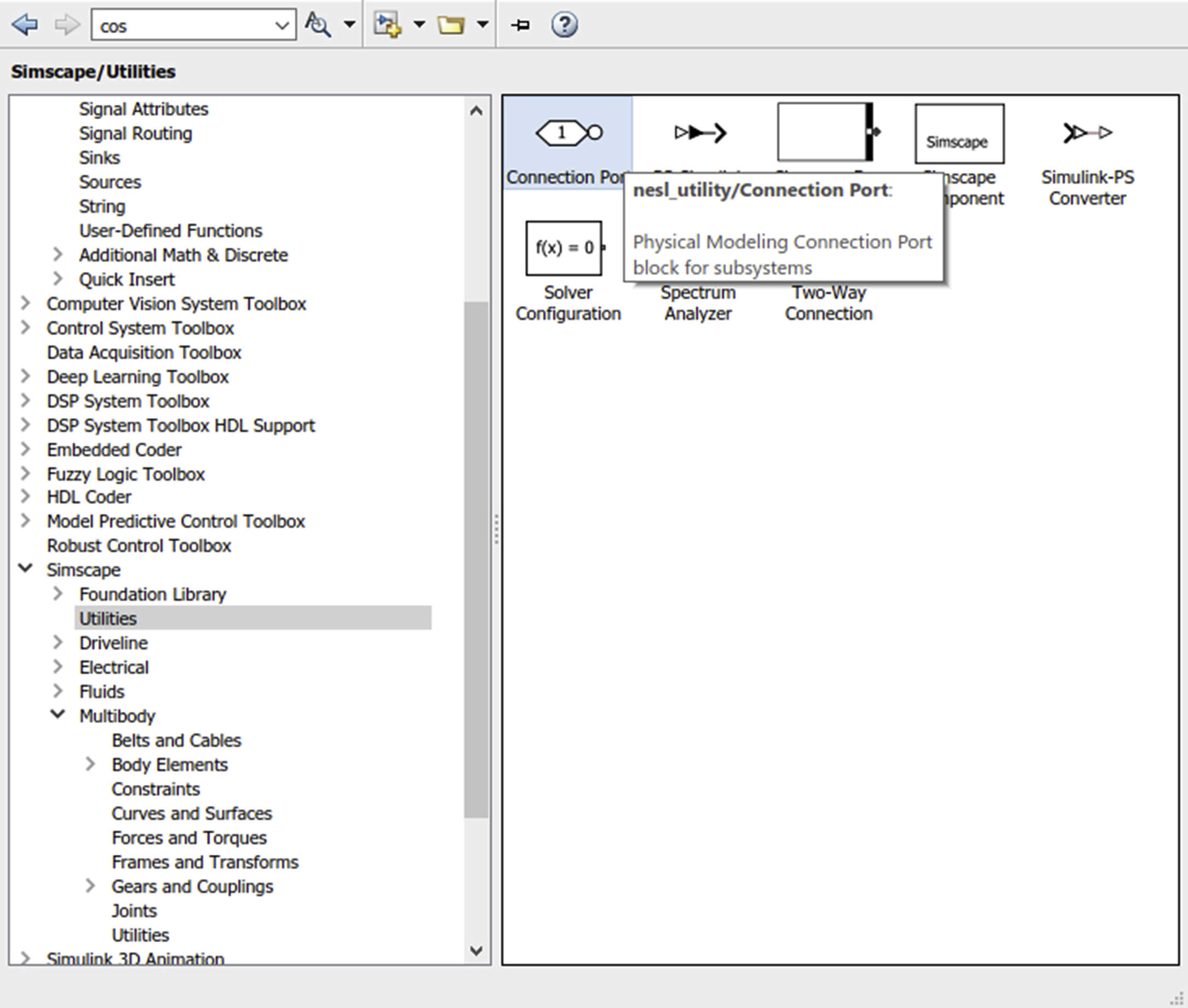
- Step 32: From Simscape>Utilities add a Connection Port (Fig. 4.30). Press Ctrl+R twice to rotate the port.
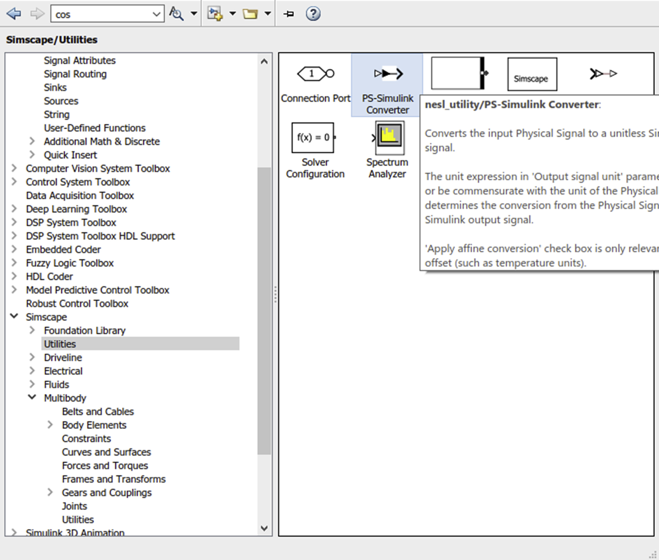
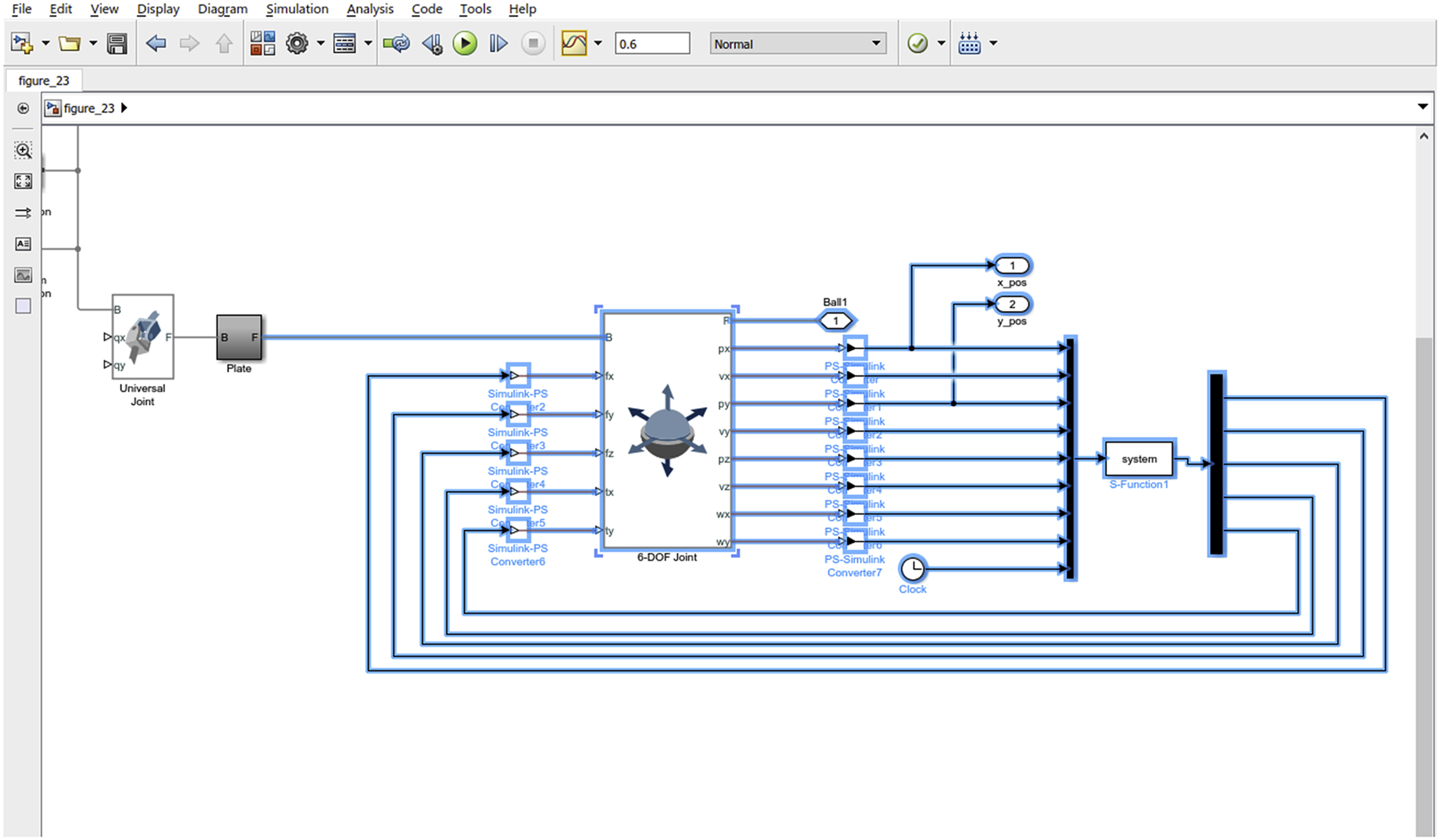
- Step 33: From Simscape>Utilities, add eight PS-Simulink Converters (Fig. 4.31).
- Step 34: Connect the F port of the 6-DOF Joint to the Connection Port. Similarly, connect px, vx, py, vy, pz, vz, wx, and wy to the PS-Simulink Converters and then to the Mux block. Fig. 4.32 shows the resulting connections.
- Step 36: Connect the S-Function block to the Demux block.
- Step 37: From Simscape>Utilities, add five Simulink-PS Converters.
- Step 38: Connect the Demux block to the five Simulink-PS Converters and connect the latter to the 6-DOF Joint block (Fig. 4.33).
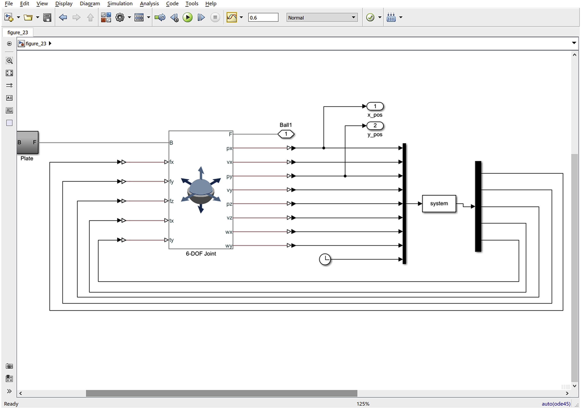
- Step 39: From Simulink>Commonly Used Blocks, add two Out1 blocks. Rename them x_pos and y_pos and connect them to px and py per Fig. 4.34.
- Step 40: Select the components highlighted in the rectangle in Fig. 4.35 and create a subsystem. Rename the subsystem Ball Plate Interaction.
- Step 41: Open the Ball Plate Interaction subsystem and rename the port Conn2 (that is connected to B) as B. Rename the port that is connected to the F port as F.
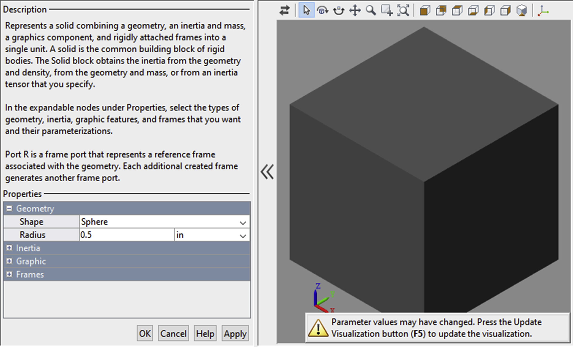
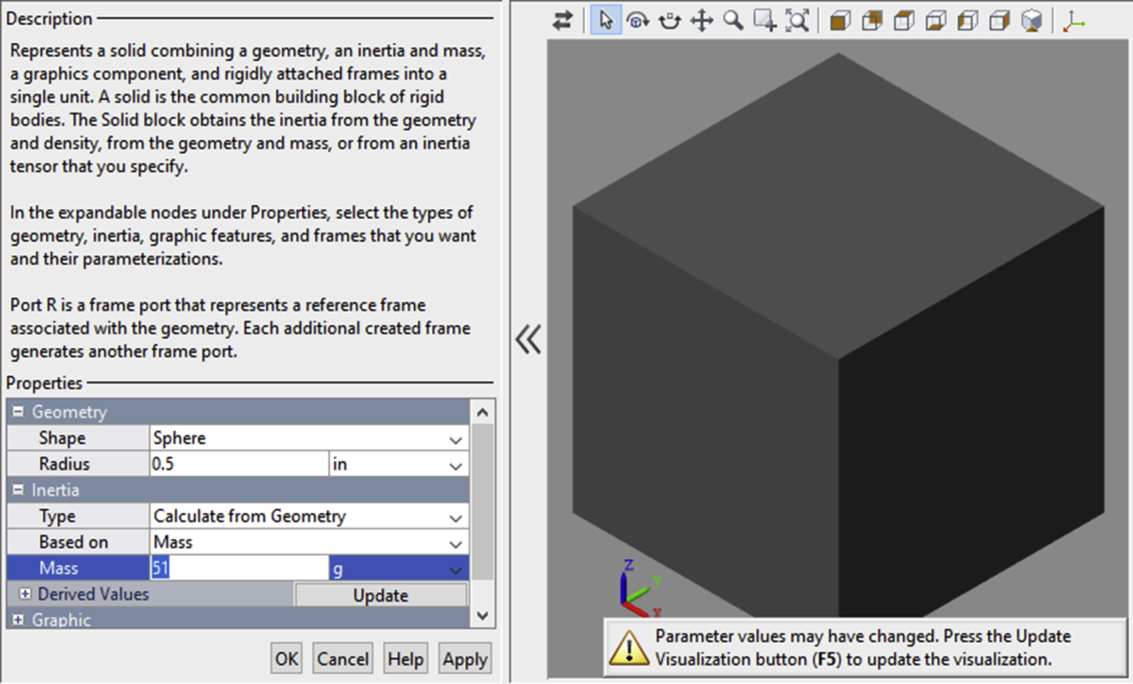
- Step 42: To create the physical object representing the ball, add the Solid block from the Simscape>Multibody Library> Body Elements Library (Fig. 4.36).
- Step 43: Rename the Solid block as Ball. Click Ctrl+R twice to rotate the Solid block.
- Step 44: Double click the Solid block. Change the shape to a sphere and the radius to 0.5 inches (Fig. 4.36).
- Step 45: Change the mass of the sphere to 51 g (Fig. 4.37). Click OK when done.
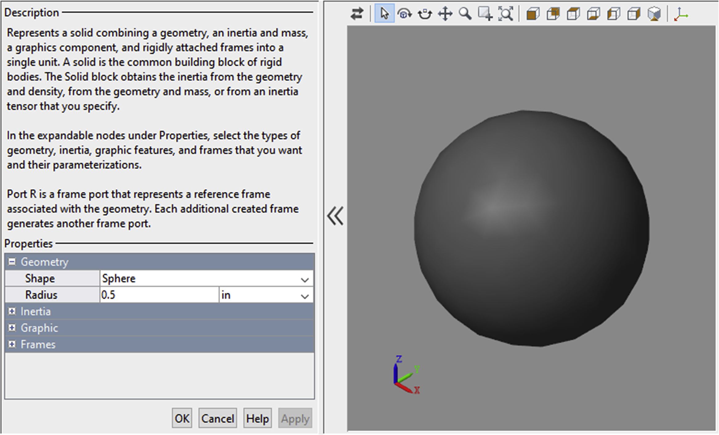
- Step 46: Double click the block and check to see the shape changed to a sphere (Fig. 4.38).
- Step 47: Delete the F port connected to the Ball port of the Ball Plate Interaction subsystem. Connect the Ball port to the Ball block (Fig. 4.39).
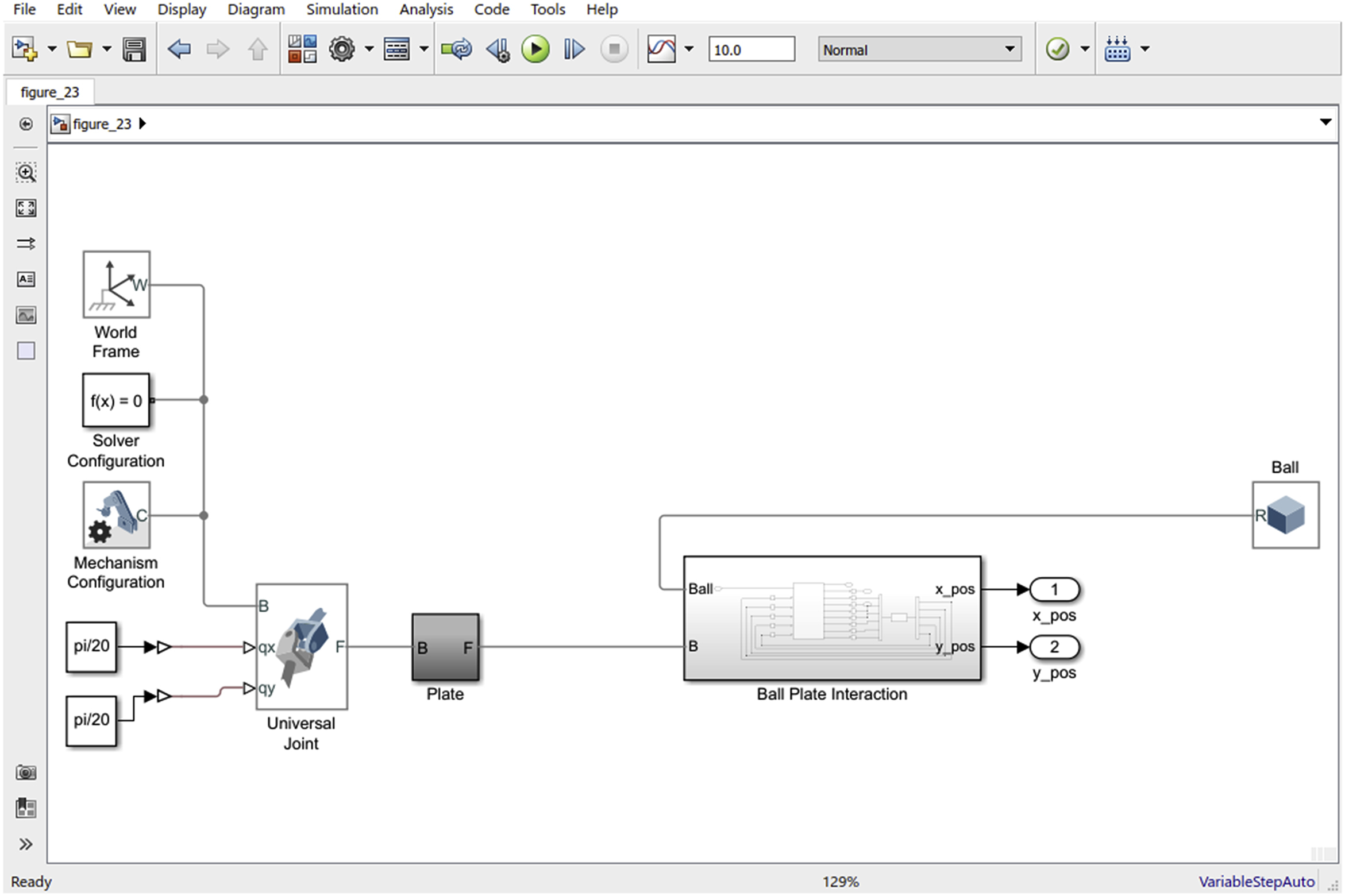
- Step 48: To add the input angles to the plate, go to Simulink>Commonly Used Blocks and add two Constant blocks. Set the value to pi/20 for both constants.
- Step 49: In order to connect the Constant to the Universal Joint, we need to add two Simulink-PS Converters like we did in step 37. Add two converters, connect the constants to the converters, and connect the later to the Universal Joint (Fig. 4.40).
- Step 50: In Simulation>Model Configuration Parameters, change max step time to 1e-3 and the simulation stop time to 0.6.
In these 50 steps, the process of adding a universal frame, frame 1 and frame 2, has been outlined. Frame 1 is attached to the plate while frame 2 is attached to the ball. The inputs to the x and y rotational angles of frame 1 are constants. In the next section, the forces of the plate on the ball will be detailed. The c-script for the s-function will be discussed.
4.6. Ball Plate Interaction
Simscape Multibody natively handles solving the interaction between the 3D components. It can solve for the forces given motion constraints, the motion using the force constraints, or a hybrid of both. The unique element of the ball on plate is that these
two 3D components are not natively connected in Simscape. This mandates calculating the interaction forces between the ball and the plate.
The first force that will be discussed is the support force that prevents the ball from sinking into the plate due to gravity (note that the force of gravity on the ball is already taken care of inherently in the solid block for the ball). This support force is the reaction force of the plate. As long as the ball is in contact with the plate, the plate will generate a force on the ball in the z direction, measured with respect to frame 1 (plate frame). This force has two components: a spring and a damper. It is an overdamped system so that the ball does not exhibit bouncing on the plate. The two components will prohibit the ball from penetrating the plate. The ball center will be distanced at
 from the center of the plate (which is where frame 1 is fixed) (Fig. 4.41). In reality, it is
hard to solve for the exact force that will keep the ball just at
from the center of the plate (which is where frame 1 is fixed) (Fig. 4.41). In reality, it is
hard to solve for the exact force that will keep the ball just at
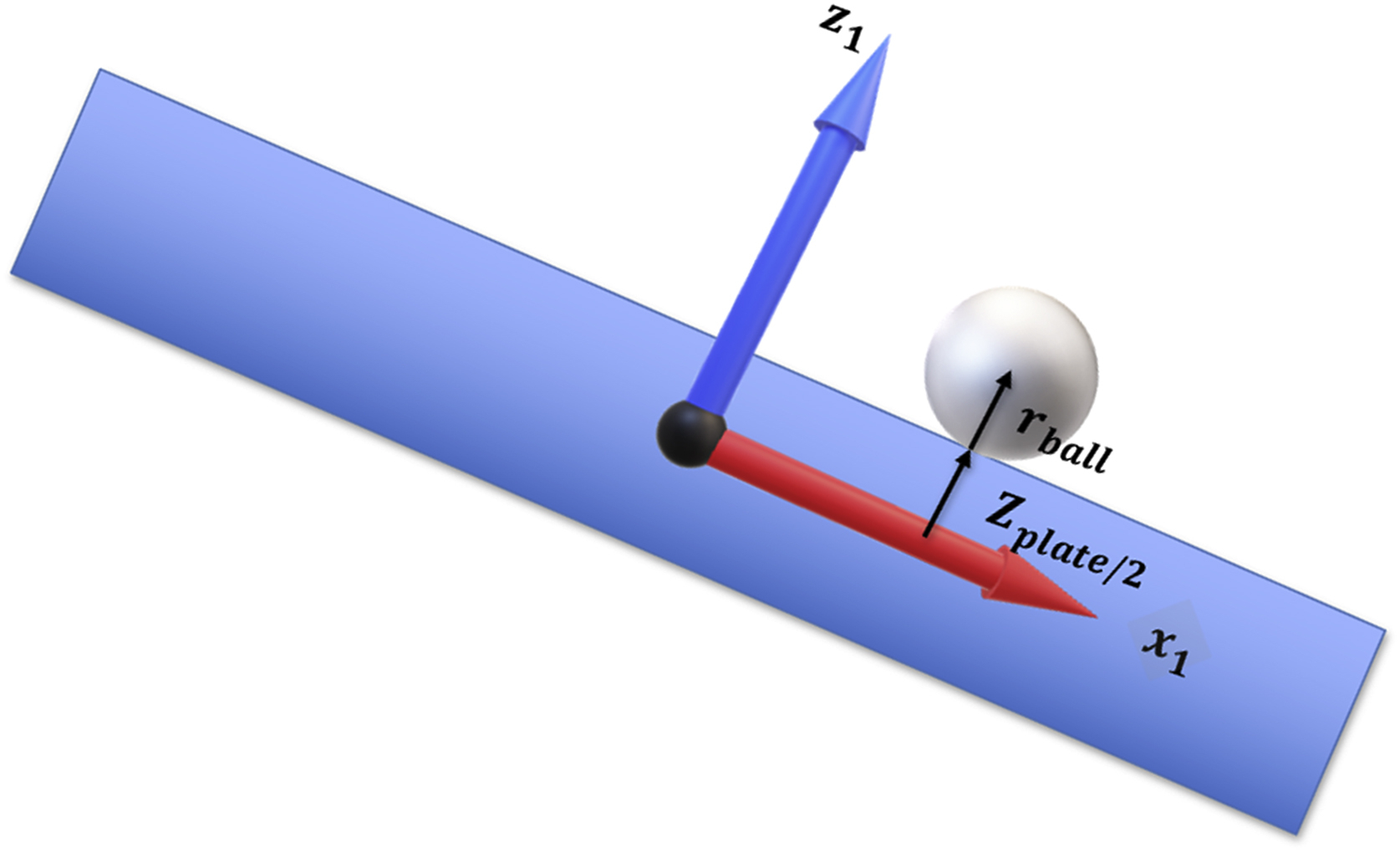
where
Note that
 will be set to zero whenever the ball is not in contact with the plate.
The remaining forces and torques that the plate exerts on the ball are the two frictions in the x and y directions and their torques.
Friction force in the x and y direction is given as
where the friction coefficient in the x and y direction is constant and is set to be
 and
and
 and
and
 are the velocities of the center of the ball in the x and y directions.
When the model is initialized, and speed of the ball is very small (practically zero), a special condition is implemented to prevent slipping of the ball on the plate. The friction coefficient
 in Eqs. (4.2) and (4.3) is replaced by
where
 and
and
 have the same direction of the friction forces and they are given by
where
 and
and
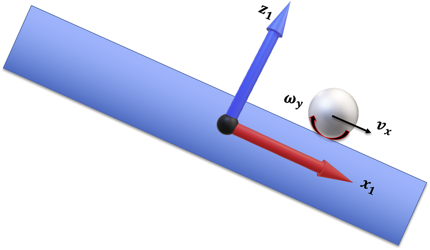
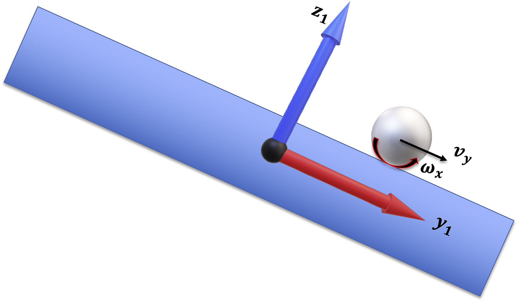
 represent the circumferential speed of the ball at point of contact with plate in the x and y directions, respectively. Using the right-hand rule of rotation, one can determine that
 is opposing the motion while
 is along the motion and thus Eqs. (4.6) and (4.7) have opposite signs.
Figs. 4.43 and 4.44 demonstrate the slippage velocities and their terms (y and x, respectively).
is along the motion and thus Eqs. (4.6) and (4.7) have opposite signs.
Figs. 4.43 and 4.44 demonstrate the slippage velocities and their terms (y and x, respectively).
The torques of these forces around the center of the ball are given by multiplying the forces by the radius of the ball.
4.7. S-function for the Ball Plate Interaction
In this section, a C-script will be constructed to calculate Eqs. (4.1)–(4.9). Start by opening a C-MEX template. Go to Simulink>User-Defined Functions>S-function Examples>C-Files>Basic C-Mex Template (Fig. 4.45). Before we write the script, we will do a minor update on the model in Fig. 4.42. Instead of six inputs to the user-defined block, we will add another input, which is the simulation time (Fig. 4.46). Below is the ballplateforces.c script with full comments explaining the implementation of the way Eqs. (4.1)–(4.9) were implemented. Script can be downloaded from MATLAB Central by searching for the book and downloading the files for this chapter. Note that you will need to type and run mex ballplateforces.c in the MATLAB® command window if you introduce any changes in the C-script or if you face any problems running the provided Simulink model.
/∗ Ball Plate Forces
∗
∗
∗/
#define S_FUNCTION_NAME    ballplateforces
#define S_FUNCTION_LEVEL   2
#include "simstruc.h"
#include <math.h>
#define PAR(element)     (∗mxGetPr(ssGetSFcnParam(S,element)))
#define U(element)      (∗uPtrs[element])
/∗ Parameters. ∗/
#define xpla          PAR(0)  /∗ Plane length [m]. ∗/
#define ypla          PAR(1)  /∗ Plane width [m]. ∗/
#define zpla          PAR(2)  /∗ Plane thickness [m]. ∗/
#define rbal          PAR(3)  /∗ Ball radius [m]. ∗/
#define Kpen          PAR(4)  /∗ Spring constant [N/m]. ∗/
#define Dpen          PAR(5)  /∗ Damping constant [N.s/m]. ∗/
#define mustat         PAR(6)  /∗ Static friction constant [ ]. ∗/
#define vthr          PAR(7)  /∗ Friction threshold speed [m/s]. ∗/
/∗ Inputs. ∗/
#define xpos    U(0)  /∗ Ball position in x-direction. ∗/
#define vx     U(1)  /∗ Ball speed in the x direction. [m/s] ∗/
#define ypos    U(2)  /∗ Ball position in y-direction. ∗/
#define vy     U(3)  /∗ Ball speed in the y direction. [m/s] ∗/
#define pz     U(4)  /∗ Ball position in the z direction. [m] ∗/
#define vz     U(5)  /∗ Ball speed in the z direction. [m/s] ∗/
#define wx     U(6)  /∗ Ball rotation speed around the x axis. [rad/s] ∗/
#define wy     U(7)  /∗ Ball rotation speed around the y axis. [rad/s] ∗/
#define Tsim    U(8)  /∗ Simulation time. [s] ∗/
/∗ Initialization. ∗/
static void mdlInitializeSizes(SimStruct ∗S) {
 ssSetNumSFcnParams(S, 8);
 if (ssGetNumSFcnParams(S) != ssGetSFcnParamsCount(S)) {
  /∗ Return if number of expected != number of actual parameters ∗/
  return;
 }
 ssSetNumContStates(S, 0);
 ssSetNumDiscStates(S, 0);
 if (!ssSetNumInputPorts(S, 1)) return;
 ssSetInputPortWidth(S, 0, 9);
 ssSetInputPortDirectFeedThrough(S, 0, 9);
 if (!ssSetNumOutputPorts(S, 1)) return;
 ssSetOutputPortWidth(S, 0, 5);
 ssSetNumSampleTimes(S, 1);
 ssSetOptions(S, SS_OPTION_EXCEPTION_FREE_CODE);
}
static void mdlInitializeSampleTimes(SimStruct ∗S) {
 ssSetSampleTime(S, 0, CONTINUOUS_SAMPLE_TIME);
 ssSetOffsetTime(S, 0, 0.0);
}
#define MDL_INITIALIZE_CONDITIONS   /∗ Change to #undef to remove function ∗/
#if defined(MDL_INITIALIZE_CONDITIONS)
 /∗ Function: mdlInitializeConditions ==============================
 ∗ Abstract:
 ∗   In this function, you should initialize the continuous and discrete
 ∗   states for your S-function block. The initial states are placed
 ∗   in the state vector, ssGetContStates(S) or ssGetRealDiscStates(S).
 ∗   You can also perform any other initialization activities that your
 ∗   S-function may require. Note, this routine will be called at the
 ∗   start of simulation and if it is present in an enabled subsystem
 ∗   configured to reset states, it will be call when the enabled subsystem
 ∗   restarts execution to reset the states.
 ∗/
 static void mdlInitializeConditions(SimStruct ∗S)
 {
 }
#endif /∗ MDL_INITIALIZE_CONDITIONS ∗/
static void mdlOutputs(SimStruct ∗S, int_T tid) {
 real_T∗y    =ssGetOutputPortRealSignal(S,0);
 real_T∗x    =ssGetContStates(S);
 InputRealPtrsType   uPtrs=ssGetInputPortRealSignalPtrs(S,0);
 real_T     cgap, Fz;
 real_T     vxslippage, vyslippage;
 real_T     mux, muy, Ffx, Ffy;
 real_T     Tx, Ty;
 /∗ Support force parameters. ∗/
 cgap=zpla/2+rbal;
 /∗ Support force Fz (eq 1) when the ball is on the plate, and simulation time is post initialization . ∗/
 if (pz<cgap && fabs(xpos)<xpla/2 && fabs(ypos)<ypla/2 && Tsim>0.001)
  Fz=-Kpen∗(pz-cgap)-Dpen∗vz;
 else
  Fz=0;
 /∗ Slippage speed(eq 6 and 7). ∗/
 vxslippage=-vx+rbal∗wy;
 vyslippage=-vy-rbal∗wx;
 if (fabs(vxslippage) <= vthr)
 /∗ Friction coefficient in the x direction(eq 4). ∗/
  mux=mustat ∗ vxslippage/vthr;
 else if(vxslippage>vthr)
 /∗ Friction coefficient in the x direction for positive velocity. ∗/
  mux=mustat;
 else
 /∗ Friction coefficient in the x direction for positive velocity. ∗/
  mux=-mustat;
 /∗ Friction force in the x direction(eq 2). ∗/
 Ffx=mux∗Fz;
 if (fabs(vyslippage) <= vthr)
 /∗ Friction coefficient in the y direction(eq 5). ∗/
  muy=mustat ∗ vyslippage/vthr;
 else if(vyslippage>vthr)
 /∗ Friction coefficient in the y direction for positive velocity. ∗/
  muy=mustat;
 else
 /∗ Friction coefficient in the y direction for positive velocity. ∗/
  muy=-mustat;
 /∗ Friction force in the y direction(eq 3). ∗/
 Ffy=muy∗Fz;
 /∗ Rolling torque around the x axis(eq 8). ∗/
 Tx=rbal∗Ffy;
 /∗ Rolling torque around the x axis(eq 9). ∗/
 Ty=-rbal∗Ffx;
 y[0]=Ffx;
 y[1]=Ffy;
 y[2]=Fz;
 y[3]=Tx;
 y[4]=Ty;
}
#define MDL_DERIVATIVES  /∗ Change to #undef to remove function ∗/
#if defined(MDL_DERIVATIVES)
 /∗ Function: mdlDerivatives ========================
 ∗ Abstract:
 ∗    In this function, you compute the S-function block's derivatives.
 ∗    The derivatives are placed in the derivative vector, ssGetdX(S).
 ∗/
 static void mdlDerivatives(SimStruct ∗S)
 {
 }
#endif /∗ MDL_DERIVATIVES ∗/
/∗ Function: mdlTerminate ============================
∗ Abstract:
∗    In this function, you should perform any actions that are necessary
∗    at the termination of a simulation. For example, if memory was
∗    allocated in mdlStart, this is the place to free it.
∗/
static void mdlTerminate(SimStruct ∗S)
{
}
/∗======================∗
∗ Required S-function trailer ∗
∗======================∗/
#ifdef  MATLAB_MEX_FILE  /∗ Is this file being compiled as a MEX-file? ∗/
#include “simulink.c"    /∗ MEX-file interface mechanism ∗/
#else
#include "cg_sfun.h"     /∗ Code generation registration function ∗/
4.8. Simulation of the model
In order to simulate the ball, we need to change the name of the script in the S-function block to ballplateforces. Additionally, set the input parameters for the script, xpla, ypla, zpla, rbal, Kpen, Dpen, mustat, and vthr to 0.35, 0.24, 0.02, 0.0254/2, 1000, 100, 0.6, and 1e-4, respectively. Once done, run the simulation. Mechanics Explorer automatically opens up to display the two geometrical bodies, the plate and the ball, along with the frames in the system. The top left display of Fig. 4.47 shows the ball at time zero is sinking into the plate. Later in the simulation, the ball transitions into the normal position on top of the plate and rolls on the inclined plate under the impact
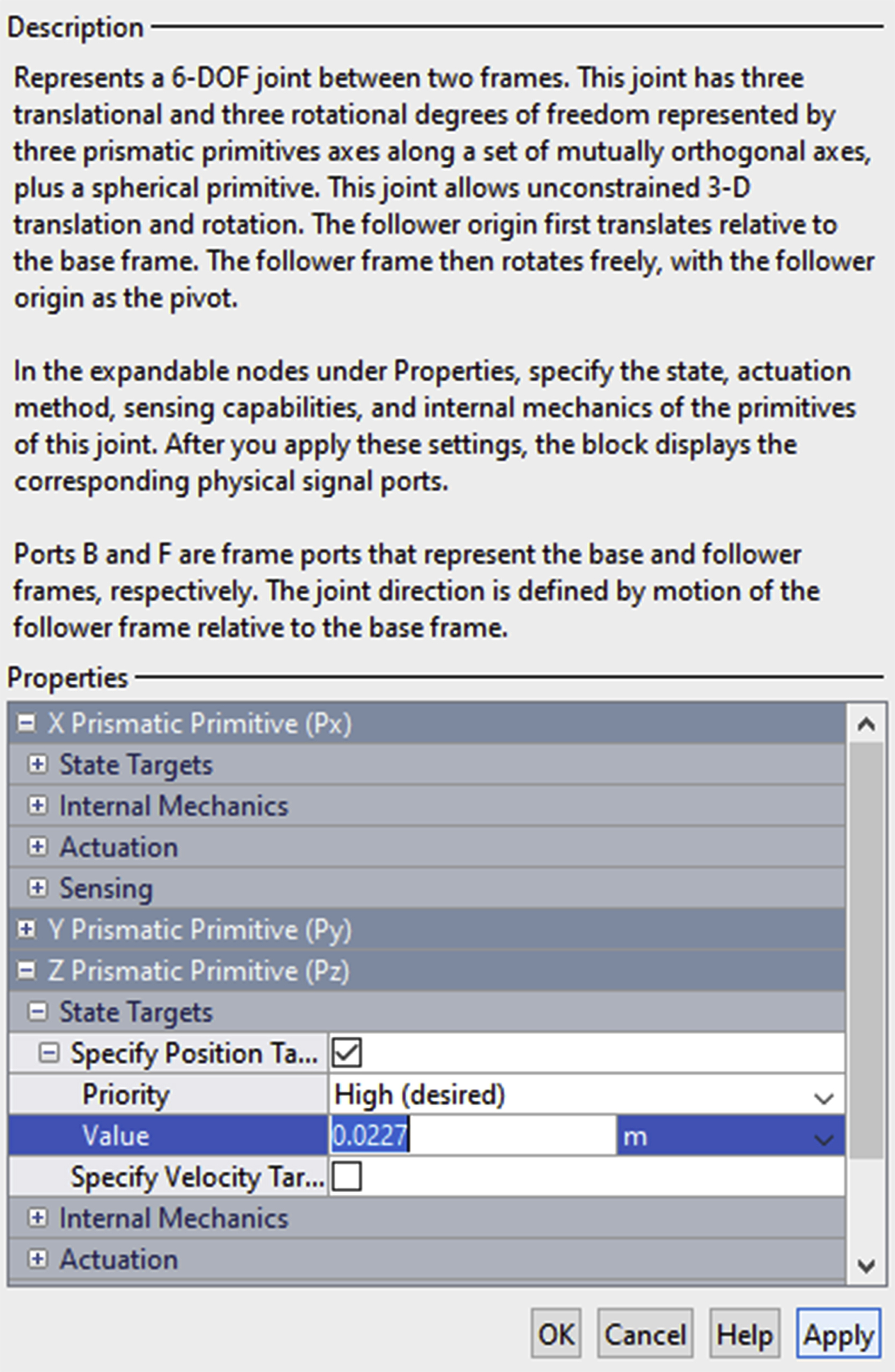
of gravity and friction. To set the initial position of the ball in the z direction, double click the 6-DOF Joint. Go to Z Prismatic Primitive (Pz)>State Targets>Specify Position Target and tick the box. Set Priority to High and Value to
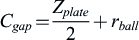 =0.02/2
+
0.0254/2=0.0227 (m) (Fig. 4.48). Click Apply and OK when done and rerun the simulation. The ball should run on top of the plate.
=0.02/2
+
0.0254/2=0.0227 (m) (Fig. 4.48). Click Apply and OK when done and rerun the simulation. The ball should run on top of the plate.
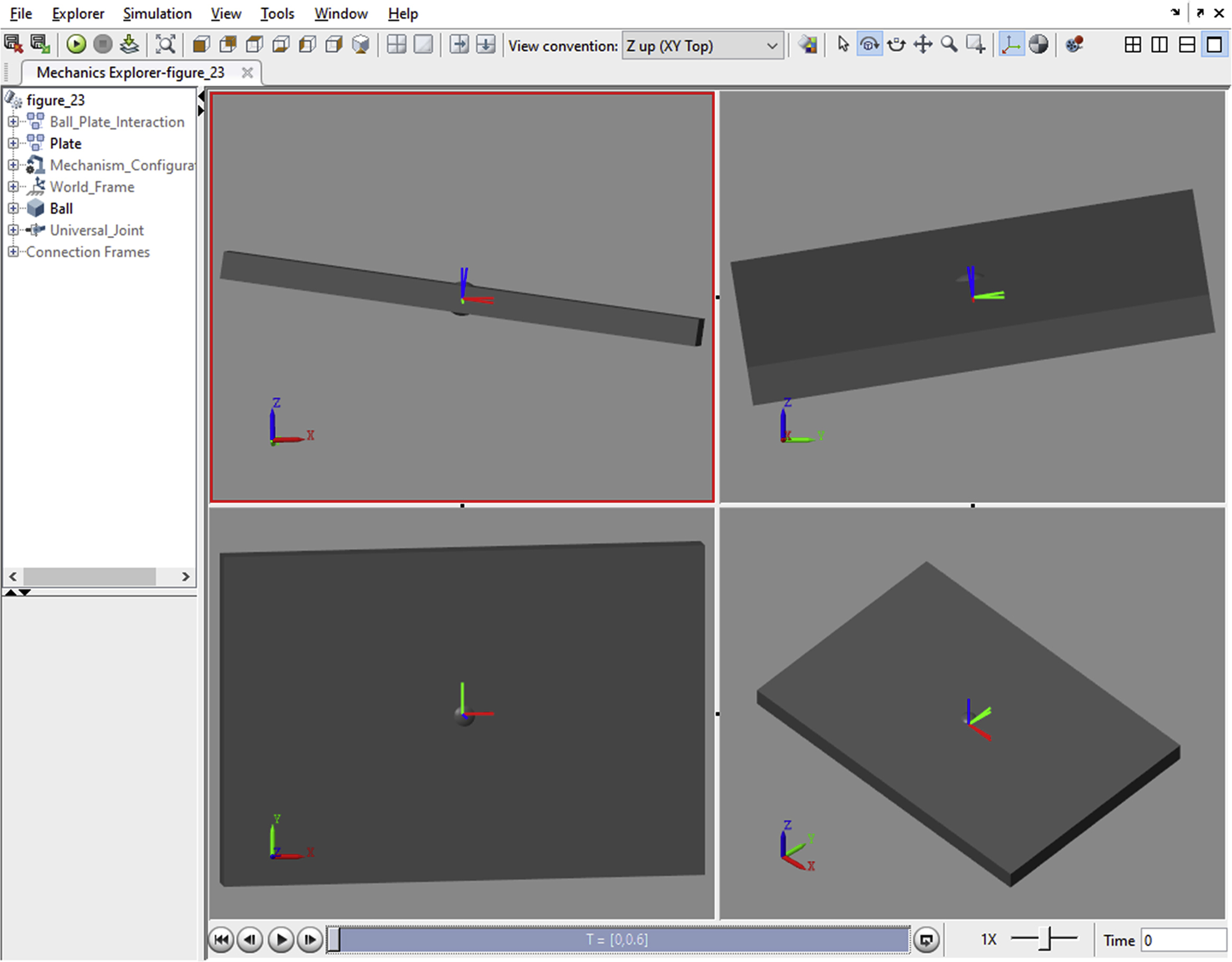
It is worthwhile mentioning that the Mechanics Explorer displays the frames of the system (axis icon on the top right corner of Fig. 4.47). It is a very helpful tool in visually checking the rotational and translational motion of the bodies.
4.8.1. Application problem 1
Given the ball on plate system in Fig. 4.1:
- (a) Develop two PID controllers for the x and y angles of the plate. The objective is to maintain the ball at the center of the plate. Simulation time is 30 s and execution time for the PID controllers is 0.01 s.
- (b) Plot the error in x, error in y, x PID output, and y PID output.
- (c) Subject the ball to an impulse force in the x-direction that is equal to 10% its weight at time=10 s. Add the force to the model and tune both PID loops. The ball needs to be within 2 cm radius of the center of the plate 7 s after the impulse (17 s from time zero).
- (d) Plot the error in x, error in y, x PID output, and y PID output.
Hint: To control the x position of the ball, you will need to manipulate qy. Similarly, to control the y position of the ball, you will need to manipulate qx. Both qx and qy are in radians.
4.8.2. Application problem 2
Replace the ball given in the chapter with square of dimensions 1.27
cm3
×
1.27
cm3
×
1.27
cm3. The x and y angles of the plate are set to
 .
.
- (a) Revisit Eqs. (4.1)–(4.9) and see if they are still applicable
- (b) Download the material for the chapter from MATLAB® Central. From folder Application_Problem_2, open ballplateforces.c and modify it according to the changes in introduced in part a. Save it as squareplateforces.c
- (c) Open ball_on_plate.slx and change the ball to a square
- (d) Type and run mex squareplateforces.c in the Matlab® command window
- (e) Change the script name in the S-Function block to squareplateforces and run the model
The final Simulink® model is provided in Application_Problem_2 folder. The Simulink® model is saved under square_on_plate.slx, and the script is saved under squareplateforces.c.
4.8.3. Application problem 3
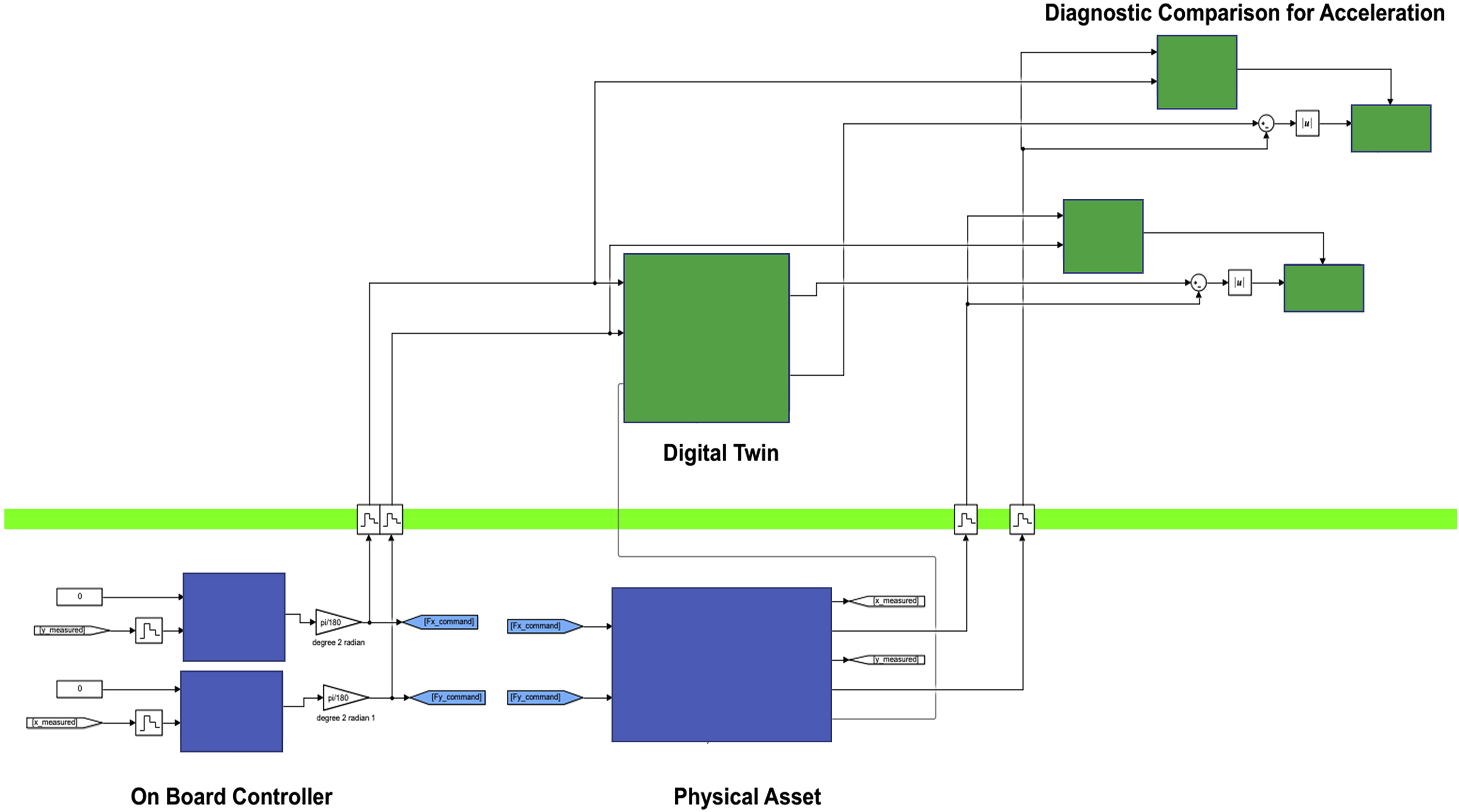
Download the material for the chapter from MATLAB® Central. In Application_Problem_3 folder, open and explore the Simulated_Digital_Twin_Good_Asset.slx model (Fig. 4.49). Notice that there are few changes introduced to the model:
- 1-the model of the plate is packaged in a subsystem for ease of readability
- 2-the output of the model is acceleration in the x and y directions instead of position. Position is still used to control the ball's position, but acceleration is used for diagnostic.
- 3-The model contains two copies of the ball on plate system: a representation of the physical hardware for the ball on plate (the lower part of the model in light blue) as well as the digital twin (the upper part of the model in green).
- 4-there are two blocks for the x and y diagnostic: one to enable the diagnostic and one to compute the deviation of acceleration between the digital twin and the physical asset.
Run the following exercises
Hint: Notice that there is a red block in the model.
..................Content has been hidden....................
You can't read the all page of ebook, please click here login for view all page.