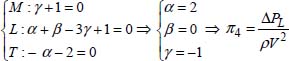
2
Dimensional Analysis: Rayleigh Method and Vaschy-Buckingham Method
2.1 Introduction
Dimensional analysis is a practical method that is used to verify the homogeneity of a physical formula through its dimensional equations and to determine the form of an equation on the basis of the hypotheses of the physical quantities on which they are based.
This method is based on the fact that only quantities of the same size can be compared or added. It provides a basis for modeling using models and for studying the effects of scale.
Dimensional analysis is applied to many problems:
- – determination of non-dimensional numbers involved in physical phenomena;
- – modeling of phenomena using models;
- – determination of scale effects.
There are many different fields where dimensional analysis can be applied, including:
- – a loss of load (or drop in pressure) in load flow;
- – flows on open surfaces;
- – aerodynamics, flow resistance;
- – the forming and propagation of waves;
- – the resistance of materials.
Dimensional analysis can be a very powerful way to obtain formulas, the literal expressions of given physical quantities, from simple intuitive reasoning.
Dimensional analysis is only an intuitive and approximate method: the accuracy of its reasoning and the results or formulas are only guaranteed to one constant.
2.2 Definition of dimensional analysis
Dimensional analysis involves applying the concept that the conditions established by the fact that the numerical value of a physical quantity depends on the system of units that has been chosen, and applying this to physical problems.
Among the set of physical quantities, it is possible to choose a subset from among them made up of the fundamental quantities, such that all other physical quantities can be expressed according to these fundamental quantities.
For mechanical quantities, the most commonly used subset of fundamental quantities are length L, mass M, and time T. These quantities are the basis of the CGS and MKS systems of units (the “International System”, or SI).
In general, a mechanical quantity G will have the following characteristics:
The numerical value of G depends on the units chosen for the fundamental quantities. The essential applications of dimensional analysis are:
- – the optimization of the experimental approach of a problem by reducing the number of parameters that must be varied to ensure the appropriate coverage of the phenomenon;
- – the verification of a relationship or equation;
- – the conversion of the numerical value of a physical quantity when changing base units.
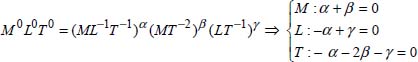
2.3 The Rayleigh method1
Lord Rayleigh devised a variant that was easier to use. If n is the number of physical quantities Gi involved in a physical phenomenon, then we can write the following:
We will express one of the physical quantities as a function of (n – 1) other physical quantities:
with:
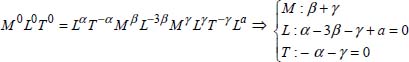
The dimension of the relationship [2.4] is:
where α, β,........,z are coefficients to be determined such that the product of the dimensions of G1,G2,.....,Gn–1 is consistent with the unit of Gi .
2.3.1 Example of application: the period of the swinging of a pendulum
Calculation of the period Tp of oscillations of a pendulum of length l and mass m in a gravitational field of g (see Figure 2.1).
The swinging of the pendulum is a physical phenomenon, and the physical quantities involved in this phenomenon are the period Tp, the length l, the mass m and acceleration of gravity g. These four physical quantities verify the following relationship:

Figure 2.1. Pendulum in oscillation: z = l(1 - cosO). For a color version of this figure, see www.iste.co.uk/sadchemloul/mechanics.zip
By expressing the period Tp according to the other physical quantities, we obtain:
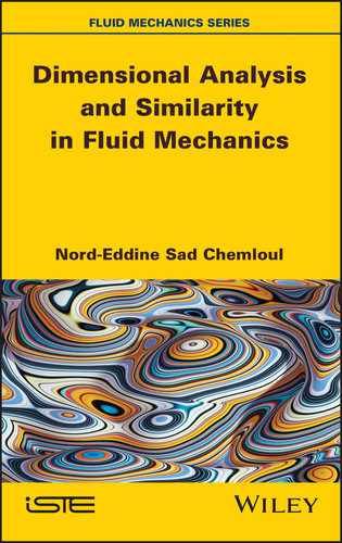
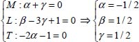
The dimension of this relationship gives us:
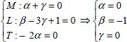
The system of equations obtained is:
The equation that gives the period of oscillation of the pendulum is:
COMMENT 2.1.- Solving the equation of the motion of a pendulum gives us a period of ![]() , which is consistent with the result found above.
, which is consistent with the result found above.
- – Recall that the equation for the motion of a pendulum is obtained from the conservation of energy, and it is given by:

- – The exact analytical expression of the oscillation period is:

with ![]() ,
, ![]() and K being a special function calledg “complete elliptical integral of the first kind”. We note that when θ0 → 0, the period Tp → T0 (see Figure 2.2).
and K being a special function calledg “complete elliptical integral of the first kind”. We note that when θ0 → 0, the period Tp → T0 (see Figure 2.2).
A pendulum twice as long will have a period ![]() times longer, and times
times longer, and times ![]() longer for a pendulum n times longer exists; this is confirmed through experience.
longer for a pendulum n times longer exists; this is confirmed through experience.
Other groupings are possible without dimensions, and this can give other dimensionless products. The most appropriate/suitable ones of these will be found through experience.

Figure 2.2. Period of oscillation of a pendulum as a function of the initial angle
2.4 Vaschy-Buckingham2 method or method of π
Non-dimensional numbers play an important role. Two questions therefore arise when considering a particular phenomenon:
- – how many “dimensional numbers” should we use?
- – how can they be determined?
The answer to the first question is given by the Vaschy-Buckingham theorem or the theory of π.
The answer to the second question is more difficult since there are several possible solutions. We need to choose the solutions that best represent the phenomenon: here, we can use certain well-known numbers as guides, such as the Reynolds number3 and the Froude number4, which translate relationships of power. Then, experience and a good analysis of the phenomenon are indispensable.
2.4.1 The Vaschy-Buckingham theorem
We will consider a physical phenomenon whose analysis makes it possible to create a list of physical quantities Gi that have an influence on this phenomenon. We can then assume that the following relationship exists:
Each of the physical quantities Gi can be expressed in a single way as a function of (n – 1) other quantities.
Or conversely f (x1,x2,...,xk) a subset of basic quantities sufficient to express the size of all quantities Gi under the form:
It is then shown that products such as:
in which Vi are the unknowns and must be dimensionless. Taking into account equation [2.7], the product [2.8] can be written as:
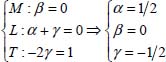
This product is therefore dimensionless if each of the exponents of the fundamental quantities is zero. We thus obtain a system of k algebraic equations containing the n unknowns Vi:
The matrix of the coefficients of the unknowns therefore comprises k rows and columns n:

We will refer to “row r” of this matrix as the number r of rows (or columns) of the largest non-zero determinant that can be deduced from this matrix.
THEOREM 2.1.– With f (G1,G2,....,Gi,....Gn) being the relationship that exists between n quantities Gi involved in the same phenomenon and k the number of fundamental quantities necessary to express the dimension of Gi.
If r is the row of matrix [2.10] constructed from the n quantities and of k fundamental quantities, the relationship f can be reduced to a relationship F(π1,π2,,π,....,πn-r) between (n – k) products with no dimensions.
COMMENT 2.3. – It should be noted that very often, row r of the matrix will be equal to the number k of the fundamental quantities, but this is not a general result.
2.4.2 Formation of terms in n
The steps to follow are:
- 1) identification of n physical quantities of the physical problem;
- 2) determination of the dimensions of each physical quantity using the basic dimensions (M,L,T);
- 3) the choice of physical quantities: these quantities must not have the same dimension (which do not form a term in π) and whose number is equal to that of the k fundamental quantities. These selected physical quantities are also called repeated quantities;
- 4) each term in π is formed by the product of these repeated quantities raised to the powers and of one of the remaining physical quantities raised to the power of one. The number of powers is equal to the number of fundamental quantities;
- 5) writing the dimension of each term in π, which makes it possible to obtain a system of equations whose unknowns are exponents of repeated physical quantities;
- 6) determination of exponents to form the terms in π and to find the relationship F(π1, π2, πi,....πn – k) = 0 .
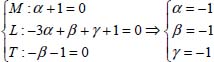
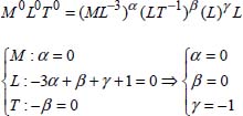
2.4.3 Application example: linear pressure drop calculation
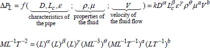
We will consider the problem of viscous flow in a round duct for the determination of a dimensionless pressure drop in accordance with other dimensionless parameters. The linear pressure drop ![]() depends on the following:
depends on the following:
- – the flow rate: the average flow rate V ;
- – the geometric characteristics of the pipe: diameter D, length Lc, the roughness of the inner wall of the pipe £ ;
- – the properties of the fluid: density ρ of the fluid, dynamic viscosity μ of the fluid.
2.4.3.1 Solution
The physical quantities involved in determining the pressure drop verify the equation:
By expressing the loss of linear load ![]() on the basis of the other physical quantities, we obtain:
on the basis of the other physical quantities, we obtain:
Procedure to follow
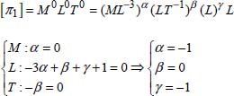
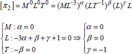
Determination of the number of physical quantities n =7.
Determination of the size of the different physical quantities:

The number of fundamental quantities is k = 3. Therefore, there are n – k = 7 – 3 = 4 terms in π, verifying the following relationship:
Choice of repeated quantities to form the terms in π: either V, D, and ρ these quantities.
Formation of terms in π

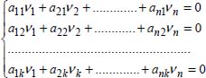
Determination of the dimension of terms in π

or:

Determination of terms in π.
Term π1:

This is the inverse of the Reynolds number, but it can be written without loss of generality as:
Term π2:
This is the ratio between the length and diameter of the pipe.
Term π3:

This is the relative roughness, which is the ratio of the absolute roughness of the pipe to its diameter.
Term n4:
This term is equal to half of the pressure coefficient, which is the ratio of the drop in pressure to the dynamic pressure. Dimensional analysis makes it possible to write the following:
The terms π verify the following relationship:
The expression of the loss of linear pressure is given by:
COMMENT 2.4.– The linear head drop or the linear head loss is therefore a function of the Reynolds number, the ratio between the length and diameter of the pipe, and the relative roughness of the pipe (ratio between the absolute roughness and the diameter of the pipe). The absolute roughness is an indication of the state of the inner surface of the pipe. It depends on the nature of the material used to make the pipe.
The relationship of the linear pressure drop would be different if the repeated quantities were different than those considered in this application. Dimensional analysis is an extremely powerful tool, but it is also very dangerous. If we forget about or make a mistake in the choice of physical variables to be considered, the results are then false. The physical sense must allow the selection of the relevant independent variables.
2.5 Exercises: homogeneity method or Rayleigh method
2.5.1 Exercise 1: Reynolds number
The Reynolds number Re is a function of the density ρ of the fluid, the flow velocity V of the fluid. and a characteristic length Lc.
2.5.1.1 Solution
The relationship between the Reynolds number and other physical quantities is:
with k being the proportionality constant.
The dimension of this expression gives us:
This system of equations is incompatible, since the number of equations is less than the number of unknowns. Thus, we must express the three exponents, α, β, and γ as a function of a, which gives us:

The expression of the Reynolds number is written as:
The values of k and a are determined experimentally.
COMMENT 2.5.– The values of k and a are determined experimentally. The exponent γ depends on rheological behavior5: Newtonian laws, plastics, pseudo-plastics, etc. For k = 1 and a = –1, we may write in a general sense:
VR and LR are the reference speed and the reference length, respectively.
The Reynolds number represents the ratio of the forces of inertia to viscous forces. In the case of a pipe with a circular cross-section, the characteristic length, also known as the reference length, represents the diameter of this section.
If the straight section of the pipe is not circular, the hydraulic diameter shall be used in calculating the Reynolds number. The hydraulic diameter is given by:
Table 2.1 shows the expression of the hydraulic diameter of sections with simple geometry for load flows and free surface flows. The reference length can thus represent a height, width, length, thickness, etc.
The Reynolds number allows us to determine the nature of the flow type: the laminar type (Re < 2100), the transition type (Re = 2100), and the turbulent type (Re > 2100) .
Rayleigh’s method provides the form of the law that determines the physical phenomenon (however, there is no evidence that the corresponding physical law exists; this is confirmed through experience). Other groupings are possible without dimensions, and this can give other dimensionless products. The most appropriate/suitable ones of these will be found through experience.
Table 2.1. Some expressions of hydraulic cross-section diameter using simple geometry. For a color version of this figure, see www.iste.co.uk/sadchemloul/mechanics.zip
| Free surface flow | Load flows | |
| Shape of cross section |  |
 |
| Cross-section area | ||
| Wetted perimeter |  |
|
| Hydraulic diameter | ||
| Shape of cross section |  |
 |
| Cross-section area | ||
| Wetted perimeter | ||
| Hydraulic diameter |
2.5.2. Exercise 2: the Weber number
Establish the expression for the Weber number We, assuming it is a function of the velocity V, the density ρ, the length Lc, and the surface tension σ
2.5.2.1 Solution
The expression of the Weber number We is written as:
with k being the proportionality constant.
Given that this number is dimensionless, the dimension of this expression gives:
The system of equations obtained is incompatible, the number of equations is less than the number of unknowns, expressing the exponents α, β, and γ, depending on a, we obtain:

The expression of the Weber number is written as:
The constant k and the exponent a determined experimentally. For k = 1 and a =–1, the Weber number is written as:
COMMENT 2.6.– The Moritz Weber6 number is a dimensionless number used in fluid mechanics to characterize the flow of fluids at the interface points of a multiphase system. It represents the ratio of inertial forces and surface tension, and thus it is written as:
It represents the relative importance of shearing forces and surface tension.
Weber’s number is primarily used for the study of the flow of films and the formation of drops or bubbles. For example, if a drop has a Weber value of greater than 12, it will disintegrate into many other small drops.
An example of the application of the Weber number is an impact on a liquid film: when an aerosol hits a surface, a liquid film may be created. Therefore, after a certain period of time, the aerosol no longer directly hits the solid surface, but a liquid film. This situation then changes the conditions of impact. This scenario is studied particularly in the context of internal combustion engines in order to model the interactions between the fuel that is injected and the cylinder walls.
Table 2.2 shows various impact regimes.
Table 2.2. Various impact regimes of drops on a liquid film
| Nature of the regime | ||
| Expression of the Weber number | The drop is captured | Partial coalescence regime |
| We < 5 | 5 < We < 10 | |
| Expression of the Weber number | Coalescence regime | Splash regime |
In this table, ρ and Vl are the density and kinetic viscosity of the liquid, dp is the diameter of the drop, and f is the frequency of the impacting drops, respectively.
2.5.3 Exercise 3: capillary number
Establish the expression of the dimensionless capillary number Ca as a function of gravitational accelerationμ, surface tension, σ and velocity dp .
2.5.3.1 Solution
The expression of the capillary number is written as:
with k being the proportionality constant.
The dimension of this expression lets us write:
For the solution of this system, the exponents α and β are expressed as functions of γ. The third equation of the system makes it possible to verify that the solutions found are exact.
The solutions to the system are:
So, we obtain:
The constant k and the exponent α are determined experimentally. For k = 1 and γ = 1, the capillary number is written as ![]()
REVIEW.- The capillary number is a dimensionless number used in fluid mechanics. It represents the ratio of viscous forces to surface tension and is used to characterize the atomization of liquids.
This number is used to evaluate the effects of surface tension, such as the study of using the propulsion of fluid film by pulling a plate or the study of dynamic angles of dampening.
The capillary number is also utilized in the rheology of fluids containing bubbles or drops (such as emulsions), to determine if these inclusions become distorted during flows.
If Ca << 1, the tension effects overpower the viscous forces, and if Ca » b the viscous forces overpower the tension effects.
The viscosity is so great that the effects of surface tension on the open surface are negligible.
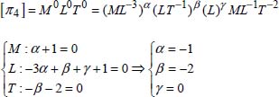
2.5.4 Exercise 4: power of a propeller
Assuming that the power ppropeller exerted by a propeller is a function of the density ρ and dynamic viscosity μ of the air, of the diameter D and rotation speed N of the propeller, the speed V of the air current, and the speed of sound c, find this expression.
2.5.4.1 Solution
The power ppropeller exerted by the propeller therefore depends on:
- – the geometric characteristics of the propeller: diameter D and speed N;
- – the properties of the fluid: density ρ and dynamic viscosity μ;
- – the speed V of the air;
- – the speed of sound c.
The expression of the power exerted by the propeller is:
with k being the proportionality constant.
The dimension of this expression gives us:
that is:

The system of equations obtained is incompatible, so we will express the exponents α, β, and γ as a function of θ, a and b, that is:

The expression of the power generated by the propeller is:
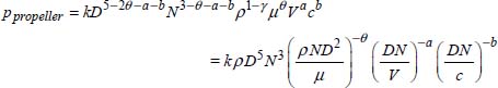
The constant k and exponents θ, a and b are determined experimentally.
For k = 1 and θ = a = b = – 1, we obtain:
COMMENT 2.7.- The term ![]() is proportional to the Reynolds number, and it can effectively be written as:
is proportional to the Reynolds number, and it can effectively be written as:
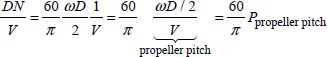
The term ![]() defines the pitch of the propeller, that is, the forward movement of the propeller after each turn. It can be written as:
defines the pitch of the propeller, that is, the forward movement of the propeller after each turn. It can be written as:
That is:
The term ![]() is proportional to the Mach number7, and it can effectively be written as:
is proportional to the Mach number7, and it can effectively be written as:
The power exerted by a propeller is therefore:
Figure 2.3 below shows an example of a propeller.

Figure 2.3. Diagram of an example of a propeller
NOTE 2.1.- A propeller is made up of at least two blades joined together around a hub, which itself is connected to a drive shaft. It can easily be noticed (see Figure 2.3) that each blade, shown in a cross section, has very obvious similarities with the wing of an airplane.
The energy output generated by the motor is transformed into forward propulsion along a straight line. Thanks to its aerodynamic properties, the propeller transforms the torque provided by the motor into a force that provides for the forward movement of the airplane through the air.
2.5.5 Exercise 5: flow through an orifice with thin walls
For a perfect liquid, express the volumetric flow Qv through a thinwalled orifice, depending on the density ρ of the liquid, the diameter d0 of the orifice and the difference in pressure ΔP.
2.5.1.1. Solution
Consider a closed tank with an orifice as shown in Figure 2.4:
where k is the proportionality constant.
The dimension of this relationship of flows is:

The solutions of the systems of equations representing the values of the exponents are:

The flow through a thin-walled orifice is:
COMMENT 2.8.– On the basis of the shape of the edges of the orifice cross section So (see Figure 2.4), we may draw a distinction between thin-walled orifices with sharp edges (see Figure 2.4a) and round-edged orifices or orifices which are machine-shaped so that the flow is properly guided by the walls (see Figure 2.4b).
The axis of the jet continues in its initial direction, but due to viscous or turbulent friction, the jet spreads out, and the velocity downstream decreases. On the basis of the contracted section or the vein Sv of the liquid, the trajectories become parallel to each other, and the pressure distribution becomes hydrostatic in nature.
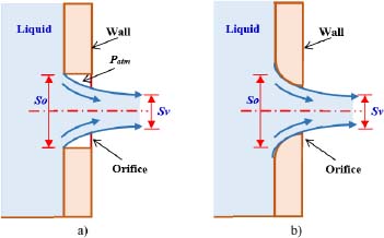
Figure 2.4. Flow through orifices: (a) a thin-walled orifice; (b) a round-edged orifice. For a color version of this figure, see www.iste.co.uk/sadchemloul/mechanics.zip
2.5.6. Exercise 6: a linear pressure drop along a horizontal pipe
Establish the expression of ΔPL, a linear pressure drop for an isovolume turbulent flow within a horizontal pipe. This pressure drop depends on the diameter D and length Lc of the pipe, the roughness ε of the inner surface of the pipe, the density ρ and dynamic viscosity μ of the fluid, and the velocity V of the flow of the fluid in the pipe.
2.5.6.1 Solution
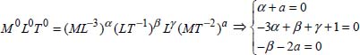
The relationship between the drop in pressure and other physical quantities is:
That is:

This system of equations is incompatible (three equations with six unknowns); the unknowns (exponents) θ, a, and b are determined based on the unknowns (exponents) α, β, and γ which are considered as fixed:

The relationship of the linear pressure drop is written as:

COMMENTS 2.9.–
The term  represents the Reynolds number:
The term  is written as:
The term  is written as:
The expression of the loss of pressure is thus given by:
The term 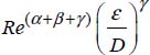 defines the coefficient of linear pressure drop λ:
which gives:
By taking α = β = γ = 1 and ![]() , we obtain the Darcy-Weisbach relationship8, which gives the linear pressure drop:
, we obtain the Darcy-Weisbach relationship8, which gives the linear pressure drop:
The coefficient λ is determined either using the ratios given in Table 2.3 or using the Moody chart9 (see Figure 2.5).
Table 2.3 gives the expressions of the coefficient of the linear pressure drop as a function of the Reynolds number and relative roughness.
Table 2.3. Expression of the coefficient of linear pressure drop λ = f (Re, ε/D)
| Regime | Re value | Expression of λ | Relationship name |
|---|---|---|---|
| Laminar | Re < 2000 | Poiseuille10 | |
| Smooth turbulent | 2000 < Re < 105 | Blasius11 | |
| Smooth turbulent | 105 < Re < 106 | Prandtl-Nikuradse12 | |
| Rough Turbulent | Re > 106 | Von Kármán13-Nikuradse | |
| Turbulent | – | Colebrook14 |
COMMENT 2.10.– The Moody chart is the representation on a single diagram of the general expression of the coefficient of the drop in pressure:
The chart was established on the basis of the theoretical studies done by Blasius and Prandtl, the numerous and well-known experiments carried out by Nikuradse (on variable roughness) and measurements made on industrial pipes.
The universal Moody diagram is shown in Figure 2.5. It provides the curves λ = f (Re) for each value of the relative roughness (![]() ).
).
Curve A represents the relationship of Poiseuille under a laminar regime (see Table 2.3).
Curves B and C represent the relationship of Blasius and Prandtl-Nikuradse when the turbulence regime is smooth (see Table 2.3).
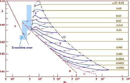
Figure 2.5. Moody diagram 
The area between curves C and G is the transition zone between hydraulically smooth and hydraulically rough flows. In this area, the coefficient of the linear pressure drop λ depends on both the Reynolds number Re and the relative roughness (![]() ).
).
The E curves, known as Nikuradse’s harp, were obtained experimentally by Nikuradse by varying both the diameter and the roughness of the pipe.
The roughness was obtained by gluing grains of sand with a well-defined granular size onto the walls of the pipe. This allowed for a uniform and very regular roughness level, both in size and distribution.
This explains the difference found in the F curves obtained by Colebrook from experiments with industrial pipes, for which roughness can vary widely. He made important contributions to fluid mechanics. He is best known for the table named after him, which provides the roughness of pipes.
Table 2.4 shows some common values of absolute roughness.
Table 2.4. Standard values of absolute roughness (ε) in mm
| Nature of the inner surface of the pipe | Absolute roughness ε (mm) |
|---|---|
| PVC | 0.0015 |
| Stainless steel | 0.015 |
| Commercial steel | 0.045 to 0.09 |
| Drawn steel | 0.015 |
| Welded steel | 0.045 |
| Galvanized steel | 0.15 |
| Rusted steel | 0.1 to 1 |
| New pig iron | 0.25 to 0.8 |
| Used cast iron | 0.8 to 1.5 |
| Cast iron | 1.5 to 2.5 |
| Sheet or asphalt cast iron | 0.01 to 0.015 |
| Well-smoothed cement | 0.3 |
| Reinforced concrete | 1 |
| Rough concrete | 5 |
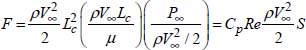
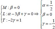
2.5.7. Exercise 7: force exerted by a fluid on a body
Given that the resistance F exerted by a moving fluid on a body is a function of the density ρ of the fluid, the dynamic viscosity μ of the fluid, the velocity at infinity V∞, the pressure at infinity P∞ of the fluid, and a characteristic length Lc of the body, establish the general equation of F.
2.5.7.1. Solution
The relationship between the strength of the resistance F and other physical quantities is written:
The dimension of this relationship is:

The expression of the resistance force is therefore:
NOTE 2.2.– In this expression:
- –
 represents twice the dynamic pressure, and
  is the surface area or master cross-section (block surface area seen from an infinite distance upstream)
  ;
; - –
 is the inverse of the Reynolds number, but it can be written without loss of generality as
  ;
; - –
 is two times the pressure coefficient, the ratio of static pressure and dynamic pressure
  .
.
By taking ![]() , θ = a = –1, we obtain:
, θ = a = –1, we obtain:
COMMENT 2.11.– The pressure coefficient is a dimensionless number that is used in aerodynamics and fluid dynamics to describe the change in relative pressure in the flow of a fluid. Each point of the flow has its own unique pressure coefficient.
The pressure coefficient is a parameter used in the study of non-compressible fluids such as water, and also in low-speed flows (flows of less than one third of the speed of sound) of compressible fluids such as air. It is given by:
Where:
- – P is the pressure at the point where the pressure coefficient is evaluated;
- – P∞ is the pressure in free flow (that is, away from any disturbances);
- – ρ is the density of the fluid in free flow;
- – V∞ is the speed of the fluid in free flow, or the speed of the body traveling through the fluid.
In many situations in aerodynamics and hydrodynamics, the pressure coefficient at a point close to a body is independent of the size of this body. Therefore, an engineering model can be tested in a wind tunnel or in a water tunnel.
The pressure coefficients can be determined at critical positions around the model and can be used to predict fluid pressure at these critical positions around an airplane or boat.
2.5.8. Exercise 8: oscillation of a liquid in a U-shaped tube
The oscillations of a non-viscous liquid in a U-shaped tube located in a vertical plane depend on the column of water Le, the density ρ, the oscillation period Tosc, and the gravitational acceleration g. Determine the relationship Tosc = f (Le, ρ, g).
2.5.8.1. Solution
The oscillation period Tosc is written as:
The dimension of the two parts of this relationship is written as:
This allows us to write:
The expression of the period of the oscillation of the liquid in the U-shaped tube is:
The value of the proportionality constant k is determined experimentally, which is k = π, and therefore:
COMMENT 2.12.– It can also be said that the oscillation of the liquid in the U-shaped tube progresses following a sinusoidal pattern:
with pulsation  , phasing φ and maximum amplitude of oscillation z0.
The period is identical to that of a simple pendulum of length ![]() . In practice, these oscillations can be observed in piezometric tubes when the pressure to be measured fluctuates slowly. The effects of friction dampen the amplitude, and the time at which a column leaves its equilibrium position is all the more difficult to determine when the amplitude is smaller.
. In practice, these oscillations can be observed in piezometric tubes when the pressure to be measured fluctuates slowly. The effects of friction dampen the amplitude, and the time at which a column leaves its equilibrium position is all the more difficult to determine when the amplitude is smaller.

Figure 2.6. Oscillation of a liquid in a U-shaped tube. For a color version of this figure, see www.iste.co.uk/sadchemloul/mechanics.zip
2.5.9. Exercise 9: a falling ball
In a fluid, a ball of radius r traveling at a speed V is subjected to a friction force given by F = – 6πμrV, where μ is the dynamic viscosity of the fluid.
- 1) What is the dimension of μ?
- 2) When the ball is released without any initial speed at the time t = 0, its speed is written as t > 0:

where a and b are constants that depend on the characteristics of the fluid. What are the dimensions of a and b?
- 3) If ρ is the density of the fluid, determine the ratio Re = ραVβμγrθ where Re is a dimensionless number.
2.5.9.1 Solutions
- 1) The dimension of dynamic viscosity is:

- 2) The falling speed of the ball is V = a(1 – e–t/b).
The argument of exponential
 is dimensionless, and thus [b] = [t] = T.
The term (1 – e–t/b) is dimensionless, and the dimension of the constant a is equal to that of the term of the velocity V:

- 3) Knowing that the dimension of the dimensionless number Re is the unit [Re] = 1 = M0L0T0, we obtain:

The exponents are given by the following ratios:

The dimensionless number is therefore written as:

For θ = –1, we find the Reynolds number:
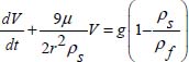
COMMENT 2.13.– A small sphere is dropped into a fluid, such as a viscometer with a dropped ball (see Figure 2.7). When the speed of the sphere becomes uniform, the balance of forces gives us:
with:
- –
 the weight of the sphere;
 - – Fν = 4μπrV the viscous force or friction between the ball and the fluid (Stokes law15);
- –
 being Archimedes’ buoyancy force16;
 - – where ρs, ρf are the density of the ball and the fluid, respectively, and r is the radius of the spherical ball.
The balance of forces gives:
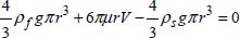
By measuring the falling speed V, we may deduce the dynamic viscosity:
This ratio is valid for a Reynolds number:
The reference length for calculating the Reynolds number is the radius of the sphere.
If Re > 5 swirls appear in the wake of the sphere, the Stokes formula is no longer applicable.
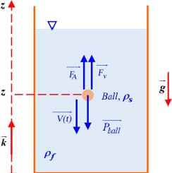
Figure 2.7. Falling ball viscometer. For a color version of this figure, see www.iste.co.uk/sadchemloul/mechanics.zip
COMMENT 2.14.– The application of the basic law of dynamics gives us:

or
With the condition of the limits V(t = 0) = 0, this differential equation has the solution:

with  .
.
The dimension of the term 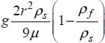 is LT–1, and that of the term
  is T–1.
In comparison with the ratio V(t) = a(1 – e–t/b) of question 2), we find:
When t → ∞, the term with the exponent tends toward 0, and the velocity V(t) tends toward a constant:
If ρf < ρs, the speed V(t) tends toward a positive value. The ball thus falls at the constant speed V∞, called the “limiting speed”.
Assuming that the ball has reached its limit speed V∞, we can use a camera to view the positions z and z + Δz of the ball at the time t and t + Δt. On the basis of the measurements of Δz and Δt, we obtain the velocity V∞, and thus the dynamic viscosity μ given by the formula:
with ![]() .
.
2.5.10. Exercise 10: implosion time of an air bubble
Find the ratio giving the implosion time tm of a water bubble that is a function of the radius r0 of the bubble, the density ρ of the water and the resting pressure p∞.
2.5.10.1 Solution
The implosion time is related to other physical quantities by the ratio:
The dimension of this relationship is:
The exponents are solutions of the following system of equations:

and therefore:
COMMENT 2.15.– The expression of the implosion time is established with the following assumptions:
- – we consider a gas bubble with a radius r0 at the time t0 and of a very low internal pressure;
- – the effects of gravity on the bubble in question and the other bubbles surrounding it are negligible;
- – the fluid around the single bubble is thus set in motion by the variations in the radius of the bubble;
- – away from the bubble considered, the speed and pressure are such that:

- – the flow of water is supposed to be perfect, non-compressible, and homogeneous, using a Galilean reference where the bubble is immobile.
NOTE 2.3.– This implosion occurs when the phenomenon of cavitation takes place. In the case of the propellers of a ship (see Figure 2.8a) that generate a significant depression, gas bubbles (water vapor bubbles) form. This phenomenon of cavitation is responsible for the erosion of the propeller (explosion of bubbles) and also creates a very characteristic noise made by the propeller (which makes it very harmful to ships).
Cavitation in water is the phenomenon of the vaporization of liquid at a temperature that remains practically constant due to the effect of a drop in pressure, generating water vapor. It is therefore clearly distinct from boiling, which takes place at a virtually constant pressure, under the effect of an increase in temperature. We may distinguish the sine wave created by the air in the water. Cavitation remains centered around the edges of the blades.
These two phenomena (cavitation and boiling) are shown schematically in the thermodynamic diagram in Figure 2.8b; the function that is shown is the vapor saturation pressure of water, the equilibrium pressure between water vapor and liquid water. Cavitation manifests itself in the formation of bubbles in areas of low pressure within a flow.
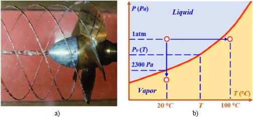
Figure 2.8. The phenomenon of cavitation and its thermodynamic diagram: a) an example of cavitation occurring on a propeller; b) thermodynamic diagram. For a color version of this figure, see www.iste.co.uk/sadchemloul/mechanics.zip
2.5.11. Exercise 11: vibration of a drop of water
The frequency of the vibration fν of a drop of water depends on several parameters. We will assume that surface tension is the predominant factor in the cohesion of the drop. Therefore, the physical quantities forming part of the expression of the frequency of vibration fν are the radius of the drop r0, the density ρ which provides the inertia, and a constant Co, which factors into the expression of the force, and which arises due to surface tension (the dimension of Co is that of a force per unit of length). Determine the expression of fv.
2.5.11.1 Solution
The vibration frequency of a drop of water is:
The dimension of the constant Co is:
The dimension of this relationship fν = f(ro, ρ, Co) is:
The exponents are solutions of the following system:

that is:

The vibration frequency is therefore written as17:

The drop of water is an oscillator characterized by its own pulsation ![]() , with σ being the surface tension of the liquid.
, with σ being the surface tension of the liquid.
COMMENT 2.16.– The cohesion of a spherical water drop is made possible by the surface tension of the drop. In this case, it will pull the drop into a spherical shape, which will therefore affect the vibration frequency of that drop. The inertia of the drop will also affect this movement, which is given by the density of the fluid.
The size of the drop is a relevant parameter, since for a larger drop of a given fluid, the cohesion is more difficult to ensure. Therefore, there is an interplay between the surface tension and the deformation of the drop during the vibration, which is taken into account in this exercise.
2.5.12. Exercise 12: drag force of water on a ship
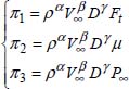
Determine the resistance force (drag force) Ft exerted by water on a moving ship, which is dependent on:
- – the length Ln of the ship, traveling at a speed V;
- – the density ρ, dynamic viscosity μ, and surface tension σ of the water;
- – the gravitational acceleration g.
2.5.12.1 Solution
The relationship that shows the relationship of the resistance force Ft exerted by water on a moving vessel is:
The dimension of this relationship is:
The exponents are solutions of the following system of equations:
Since this system is incompatible, the exponents α, β, and γ are determined according to the other exponents, that is:

The expression of the drag force is therefore:
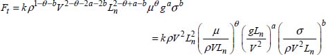
NOTE 2.4.– The term ![]() is the inverse of the Reynolds number:
is the inverse of the Reynolds number:
The term ![]() is the inverse of the square of Froude’s number:
is the inverse of the square of Froude’s number:
The term ![]() is Weber’s number:
is Weber’s number:
The term ![]() is the front surface of the ship, known as the “Master cross section”.
is the front surface of the ship, known as the “Master cross section”.
The water drag on the ship is written as:
COMMENT 2.17. – The drag force therefore depends on three-dimensional numbers:
- – the Reynolds number “Re” shows the effect of the forces of viscosity, or the influence of drag forces from water on the ship’s hull;
- – the Froude number “Fr” shows the effect of the forces of gravity or the influence of the wake, that is, the influence from the system of waves produced behind the vessel;
- – the Weber number “We” shows the effect of forces of surface tension, which are negligible in this case.
2.6. Exercises: Vaschy-Buckingham method or method of π
2.6.1. Exercise 13: pressure drop in a pipe of circular cross-section
Consider a fluid of density ρ and dynamic viscosity μ flowing at speed V in a horizontal pipe of diameter D. The average height of irregularities considered as roughness (absolute roughness) in this tube is ε. In considering two straight sections of the pipe at a distance of a length of Lc, determine the expression of the linear pressure drop ΔPL between the two sections.
2.6.1.1. Solution
The physical quantities involved in determining the drop in pressure ΔPL in the flow (see Figure 2.9) are:
- – characteristics of the pipe: Lc, D and ε;
- – the fluid’s properties: ρ and μ;
- – flow speed: V.
The number of physical quantities, including the pressure drop, is n = 7.
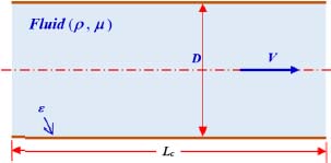
Figure 2.9. Pressure drop in horizontal pipe of circular cross-section. For a color version of this figure, see www.iste.co.uk/sadchemloul/mechanics.zip
The dimension of these physical quantities is:

The number of fundamental quantities is k = 3.
The number of terms π involved in determining the pressure drop is n – k = 7 – 3 = 4.
For the formation of terms in π the selected or repeated quantities are ρ, V and D, that is:

We will consider the dimensions of terms in π:
The term ![]() is the ratio between the length and diameter of the pipe.
is the ratio between the length and diameter of the pipe.
The term ![]() is the relative roughness: the ratio of the absolute roughness of the inner surface of the pipe to the diameter of the pipe.
is the relative roughness: the ratio of the absolute roughness of the inner surface of the pipe to the diameter of the pipe.
The term ![]() represents the inverse of the Reynolds number; a dimensional analysis allows us to write
represents the inverse of the Reynolds number; a dimensional analysis allows us to write ![]() .
.
The term  is the relationship between the pressure drop and the dynamic pressure, which is the pressure coefficient.
The terms in π thus verify the expression:
The expression of the loss of pressure is thus given by:
NOTE 2.5.– As the relationship ![]() is constant for all straight pipes with circular cross-sections, the pressure drop is therefore written:
is constant for all straight pipes with circular cross-sections, the pressure drop is therefore written:
The function ![]() is called the “linear pressure drop coefficient”. This coefficient depends on the flow regime (Reynolds number Re) and the relative roughness
is called the “linear pressure drop coefficient”. This coefficient depends on the flow regime (Reynolds number Re) and the relative roughness ![]() . The determination of λ is created from the relationships in Table 2.3 or from the Moody diagram in Figure 2.5 of exercise 6.
. The determination of λ is created from the relationships in Table 2.3 or from the Moody diagram in Figure 2.5 of exercise 6.
2.6.2. Exercise 14: friction forces on a flat plate
Determine the relationship giving the friction (or drag) force Ft exerted by a fluid moving at a speed of V on a flat plate of length Lp and width lp. The flow occurs parallel to the length of the plate. The fluid has a density of ρ and a dynamic viscosity of μ.
2.6.2.1. Solution
The physical quantities are: the friction force Ft, the velocity of the fluid V, the plate length Lp and width lp, the density ρ and the dynamic viscosity μ of the fluid, that is, n = 6.
The dimensions of these physical quantities are:
The number of fundamental quantities is k = 3.
The number of terms in π is n – k = 6 – 3 = 3. For the formation of terms in π the quantities chosen are ρ, V and Lp:
The dimension of the term π1 gives us:

The expression of the term π is  .
.
The dimension of the term π2 gives us:
The expression of the term π2 is  , which is the ratio of the width to length of the flat plate.
The dimension of the term π3 gives us:

The expression of the term π3 is  , which is the inverse of the Reynolds number Re.
Dimensional analysis makes it possible to write the following: ![]()
The terms in π thus verify the expression:
The expression of the frictional force is 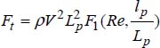 .
.
COMMENT 2.18.– The ratio ![]() is constant for all flat plates (with similar geometrical forms).
is constant for all flat plates (with similar geometrical forms).
The force of friction on both sides of the plate is written as:
In this relationship, the product Lplp represents the area of a single face of the plate (Splate = Lplp).
For one side of the plate ![]() .
.
The relationship ![]() is the stress along the wall and the relationship
is the stress along the wall and the relationship ![]() is the coefficient of friction (or drag coefficient) that is dependent on the Reynolds number. The term ρV2/2 represents the dynamic pressure, and thus the coefficient of friction (or drag coefficient) is the relationship between the shear stress along the wall and the dynamic pressure.
is the coefficient of friction (or drag coefficient) that is dependent on the Reynolds number. The term ρV2/2 represents the dynamic pressure, and thus the coefficient of friction (or drag coefficient) is the relationship between the shear stress along the wall and the dynamic pressure.
The stress measured on the wall depends on the position x taken, τp(x), on the length of the plate (direction of the flow), and thus we may refer to the local coefficient of friction:
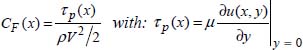
with u(x, y) being the speed profile inside the boundary layer.
Upstream of the flat plate, the fluid has an infinite upstream velocity of U∞. The flow of the fluid is parallel to the plate, the thickness of which is generally considered negligible along its leading edge (see Figure 2.10). Outside the boundary layer, the velocity of the fluid remains constant at the value of U∞, which is the region of the free stream where the inertial forces are very large with respect to the viscous forces. Inside the boundary layer, the viscous forces are greater than the inertial forces, and the velocity gradient is not zero.
The thickness δ(x) of the boundary layer of x is defined as:
In the case of the laminar boundary layer, the momentum transfer is ensured by the viscous friction within the entire boundary layer. The local coefficient of friction varies as given by ![]() (Rex is the Reynolds number determined along the axis of x), and the local tangential stress decreases as we move away from the leading edge of the plate.
(Rex is the Reynolds number determined along the axis of x), and the local tangential stress decreases as we move away from the leading edge of the plate.
In the turbulent boundary layer, the transport of the quantity of movement is only provided by the viscous friction within a very thin sublayer, known as the laminar boundary layer. Above this layer, the transport of the amount of movement is provided by turbulent lateral fluctuations. The local coefficient of friction is essentially independent of the position x taken on the plate, and the drag coefficient is nearly constant. This result shows that the drag coefficient is independent of the Reynolds number in the turbulence scheme, which means that the drag force varies at the level of ![]() .
.
In the general case, the velocity at infinity U∞ is different from the speed Ue outside the boundary layer of turbulence.
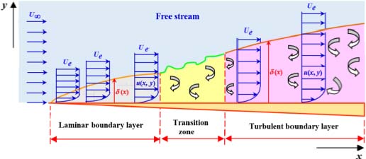
Figure 2.10. Flow near a flat wall (dynamic boundary layers). For a color version of this figure, see www.iste.co.uk/sadchemloul/mechanics.zip
2.6.3. Exercise 15: drag force exerted on a sphere
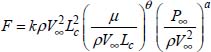
Determine the relationship of the drag force Ft exercised by the uniform flow of a non-compressible viscous fluid over a sphere. This drag depends on the density ρ and dynamic viscosity μ of the fluid, the speed and pressure at infinity of the flow, V∞ and P∞, and the diameter of the sphere.
2.6.3.1 Solution
The drag Ft exerted on an object is expressed as:
The number of physical quantities is therefore n = 6.
The dimension of these physical quantities is:
The number of fundamental quantities is k = 3 . Thus, there are three (n – k = 3) terms in π.
The quantities that are repeated (or chosen) in the formation of the terms in π are ρ, V∞, and D:
The dimension of the term π1 gives us:
The expression of the term π1 is ![]() .
.
The dimension of the term π2 gives us:
The expression of the term π2 is ![]() . This is the inverse of the Reynolds number, but we can write it as:
. This is the inverse of the Reynolds number, but we can write it as:
This is allowed in dimensional analysis.
The dimension of the term π3 gives us:
The expression of the term π3 is ![]() .
.
The three terms in π thus verify the expression:
The drag is given by the relationship:
NOTE 2.6.– The pressure P∞ has an effect on determining the momentum balance through its gradient; this field is defined to within a constant. Therefore, any translation of the value P∞ leaves the drag force Ft as fixed. It then follows that Ft is independent of the non-dimensional quantity ![]() . The drag can only be expressed as a function of the only dimensional number, which is the Reynolds number Re, giving us:
. The drag can only be expressed as a function of the only dimensional number, which is the Reynolds number Re, giving us:
In practice, the drag force is given in the following form:
with CD being the drag coefficient, dependent on the Reynolds number, CD = F(Re), S = πD2/4 being the apparent surface area of the sphere in the direction of the flow, and ![]() being the dynamic pressure. This empirical result is supported by analytical and experimental studies. In effect, an analytical development based on the theory of potential flows shows us that for flows with very low Reynolds numbers (Re ≈ 1), the drag coefficient is expressed analytically in the following way:
being the dynamic pressure. This empirical result is supported by analytical and experimental studies. In effect, an analytical development based on the theory of potential flows shows us that for flows with very low Reynolds numbers (Re ≈ 1), the drag coefficient is expressed analytically in the following way:
On the other hand, experimental work shows that for the larger Reynolds numbers, the variation of CD can be shown by what is presented in Figure 2.11. This figure shows that for a Reynolds number 103 < Re < 2 × 10⁵, the coefficient CD maintains a largely constant value, independently of Re, and around the value q.44.
For a Reynolds number of the order of Re = 3 × 10⁵, the value CD drops sharply. This fall is due to the drag crises phenomenon.
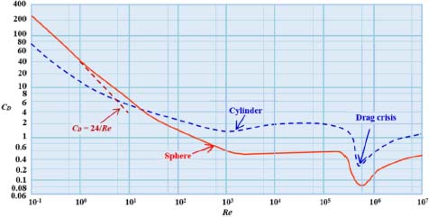
Figure 2.11. Variation of the drag coefficient as a function of the Reynolds number in the case of a sphere and a cylinder. For a color version of this figure, see www.iste.co.uk/sadchemloul/mechanics.zip
CONCLUSION.– The dimensional analysis for this study scenario has allowed us to simplify the study considerably. Effectively, it showed that the drag depends on a single, non-dimensional parameter: the Reynolds number. More in-depth studies (analytical or experimental studies) allow us to better explain such a relationship.
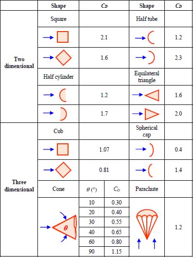
For commonly used non-spherical obstacles, Table 2.5 gives the drag coefficient values measured experimentally for some commonly used two-dimensional and three-dimensional objects, and for a range of Reynolds numbers greater than 104.
Table 2.5. Drag coefficient values for two-dimensional and three-dimensional objects calculated on the front surface area for a Reynolds number greater than or equal to 105. For a color version of this figure, see www.iste.co.uk/sadchemloul/mechanics.zip
2.6.4. Exercise 16: hydraulic jump
In a channel with a horizontal bottom, a study is to be conducted of linear geometric characteristic X of a jump in the hydraulic flow formed by the liquid flowing under a canal gate with height a subjected to a load H, with the runoff downstream having the value of y. Conduct a dimensional study of the problem, neglecting the viscosity forces and the surface tension.
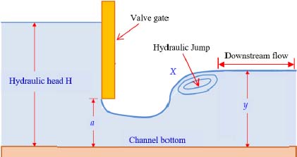
Figure 2.12. Flow in a channel. For a color version of this figure, see www.iste.co.uk/sadchemloul/mechanics.zip
2.6.4.1 Solution
REVIEW.– In flows on open surfaces (see Figure 2.12), the effects of viscosity are often negligible. In addition, the effects of surface tension are too small in comparison with the effects of gravity.
Thus, the factors having an effect are: the load H, the lifting of the gate a, the water flow y downstream of the gate, the gravitational acceleration g, and the density ρ.
The linear geometric characteristic X is written as:
The number of physical quantities is therefore n = 6.
The dimension of these physical quantities is:
The number of fundamental quantities is k = 3.
The number of terms π involved in determining the pressure drop is n – k = 3.
For the formation of terms in π the quantities chosen are ρ, g, and H, which gives us:

NOTE 2.7.– This system is formed from the same equation, because X, a and y have the same dimension.
The dimension of the three terms in π is:

These three terms in π verify the relationship:
COMMENT 2.19.– It should be noted that the Froude number does not have any effect when it is a flow on an open surface where the inertial forces and gravitational forces have a great influence. In reality, the relationships of ![]() and
and ![]() are equivalent to Froude numbers, because the speed arising from the load H on the valve is proportional to
are equivalent to Froude numbers, because the speed arising from the load H on the valve is proportional to ![]() (the Torricelli ratio).
(the Torricelli ratio).
The result obtained shows that the physical quantities ρ and g have no direct influence on the physical phenomenon of the hydraulic canal gates. The gate is the main means used by hydraulic structures to dissipate energy. It is formed during the abrupt transition from a torrential flow (or super-critical flow) to streaming flow (or sub-critical flow). During this transition, a stationary wave is formed and the energy is then dissipated through turbulence.
Thus, one of the important roles of these works is to convert the flow of the stream (usually a runoff flow) to a torrential flow, so that the gate of the water jump can be formed. This is achieved either through a flow on an inclined slope higher than the critical slope (inclined fall), or through the free fall of a body of water (vertical fall). In order to attain the correct size of these hydraulic works, it is essential to have correct knowledge of the characteristics of the water drops. This primarily includes the water levels upstream and downstream of the drop-off, and the length necessary for the completion of this drop.
2.6.5. Exercise 17: flow through a thin-walled spillway with a horizontal crested
Using dimensional analysis, find the formula giving the flow Qv of a spillway with thin walls and a horizontal limiter. This flow depends on the width of the spillway B, the upstream height of the water H, and the gravitational acceleration g. We will not consider viscosity and surface tension.
2.6.5.1 Solution
The effects of viscosity and surface tension are negligible, only inertia and gravity forces will be considered, and the volumetric mass ρ of the liquid will be eliminated. The relationship of the flow rate is written as Qv = f(B, H, g), and the number of physical quantities is n = 4.
The dimension of the physical quantities is:
The number of fundamental quantities is k = 2, that is, two terms in π:

We will consider the dimensions of π terms in:
and therefore ![]() .
.
and therefore ![]() .
.
Therefore, we can write:
The expression of the flow rate Qv of a thin-walled spillway with a horizontal limiter is:
COMMENT 2.20.– We can solve this problem by considering the volume flow per unit width Qv/B, which depends on the height of the water H above the limiter and the gravitational acceleration g.
The relationship of the flow is written as:
The number of physical quantities to take into account is n = 3.
The dimension of physical quantities is:
The number of fundamental quantities is k = 2. One can thus form a single non-dimensional product which is equal to a constant K:
The dimension of this term gives us:

or:
The constant K has no dimension and will be determined from experience or from considerations outside of dimensional analysis.
When considering similar spillways geometrically, the function ![]() of the relationship [2.12] is linear, that is
of the relationship [2.12] is linear, that is ![]() .
.
The relationship [2.12] is thus written as:
We obtain the relationship [2.13].
Weirs are devices used to measure and control runoff flow rates. They have other uses than for measuring flows. In rural areas, weir barriers are used for water management and floodwater rerouting.
Protective weirs allow for excess flow levels to be redirected when dams are in danger.
Weirs consist of a wall, which can be either thin or thick, placed vertically and left open along the top. This opening is often rectangular, triangular, as we will examine in the next exercise, trapezoidal, or parabolic.
2.6.6. Exercise 18: flow through a triangular weir
Using dimensional analysis, find the formula giving the flow Qv through a triangular spillway with thin walls as a function of the water height H, a spillway width B and a gravitational acceleration g. We will not consider the viscosity of the fluid and the surface tension.
2.6.6.1. Solution
The number of physical quantities is therefore n = 4.
The dimension of physical quantities is:
The number of fundamental quantities is k = 2. Thus, there are two terms in π.
If g and H are taken as chosen or repeated quantities, the terms π are written as:

The dimension of the terms π gives us:
and therefore ![]() .
.
and therefore ![]() .
.
The expression of the flow is ![]() .
.

Figure 2.13. Dimensions of a triangular spillway. For a color version of this figure, see www.iste.co.uk/sadchemloul/mechanics.zip
COMMENT 2.21.– If the effects of viscosity and surface tension are negligible, only inertia and gravity forces will be considered, and the volumetric mass of the liquid will be eliminated.
The height H is counted positively above the top of the spillway. We can also find the following solution:

The expression of the flow is:
The function F1(θ) has no dimension and will be determined from experience or from considerations outside of dimensional analysis. This function is proportional to that obtained in the first solution:
because:
The general flow formula for a thin-walled triangular spillway is:
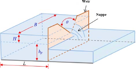
Figure 2.14. Triangular notch weir with thin wall, placed in a hydraulic channel. For a color version of this figure, see www.iste.co.uk/sadchemloul/mechanics.zip
Cd is the flow coefficient that depends on the type of spillway (shape and size). It represents all parameters (see Figure 2.14) that influence the flow, including:
- – the angle of the opening θ or angle at the peak;
- – the height of the overflow wall hp, also called the “scoop height”;
- – the water load H above the edge of the wall, measured before the sagging of the surface occurs once the flow arrives;
- – the flow supply width of channel B;
- – the total length of the flow supply of channel L.
2.6.7. Exercise 19: volume of a bubble
Considering that the volume υ of a bubble formed slowly within a liquid out of an orifice with a fairly small diameter only depends on the volumetric weight ϖ of the liquid, the liquid’s surface tension σ, and the dynamic viscosity μ. Under these conditions, give the expression of this volume.
2.6.7.1. Solution
The number of physical quantities is therefore n = 4.
The dimensions of these physical quantities are:
The number of fundamental quantities is k = 3.
So there is only one term in π, which is n – k = 4 – 3 = 1.
If, ϖ, σ, and μ are taken as chosen or repeated quantities, the term π is written as π = ϖασβμγυ.
The dimension of this term gives us:
The term in π is written as 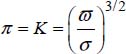 υ with K being constant. The expression of the volume of the bubble is
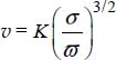
NOTE 2.8.– The same solution can be obtained by assuming that the forming of the bubble is done very slowly, and therefore the effect of dynamic viscosity is negligible. In this case, the problem becomes almost static, and it is advisable not to introduce time units.
By choosing force as the fundamental unit, the three variables υ, ϖ, and σ can only be expressed according to the two fundamental units of force and length:
Thus, there is only one term in π, which is:
And thus, the relationship can be written as:
with K1 = (K)3/2 as a constant.
The forming of the bubble created slowly in a liquid through a fairly small diameter orifice depends on the following:
- – the geometric criterion: if
 , the formation of bubbles is made through a constant flow, with d and L being the diameter and length of the orifice, respectively;
 - – the criterion based on the drop in pressure ΔP between the inside and outside of the bubble. It is necessary to have
 in order for the bubble to form.
The volume of the bubbles increases with the flow of the liquid within which the bubbles form.
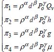
2.6.8. Exercise 20: flow through an orifice
A container holds a liquid of density ρ at a height h and viscosity μ, above which it will have the pressure Po. Through an orifice with diametered and sharp edges, a volume flow Qv flows toward the outside, which is assumed at zero pressure.
Assuming a size h before d, what form of the law would give Qv?
2.6.8.1. Solution
The number of physical quantities is therefore n = 7.
The dimension of the physical quantities is:
The number of fundamental quantities is k = 3, that is, four terms in π:
Or ρ, d, and Po, the quantities repeated or chosen.
The terms in π that are formed are:
The dimension of the term π1 gives us:

The term π1 is written as  .
.
The dimension of the term π2 gives us:


Figure 2.15. Determining the volumetric flow through an opening; Patm designating atmospheric pressure. For a color version of this figure, see www.iste.co.uk/sadchemloul/mechanics.zip
The term π2 is written as ![]() , but considering experience, we may write
, but considering experience, we may write ![]() .
.
The dimension of the term π3 gives us:
The term π3 is written as ![]() .
.
Considering the physical aspect of pressure, the physical quantity d is replaced with h.
Taking the experience into account, we may write:
The dimension of the term π4 gives us:
The term π4 is written as ![]() .
.
Taking the experience into account, we may write:
The terms in π are linked through:
The law that gives the flow is therefore written as:
Taking into account that h is very large in comparison with d, we may conclude that the relationship ![]() has no effect on the results, and therefore:
has no effect on the results, and therefore:
COMMENT 2.22.– There is another solution to the problem. It can be considered that the flow Qv is only a function of the pressure distribution that exists around the orifice, which is:
Therefore, the physical quantities involved are Qv, d, Po, ρ and μ. The number of terms in π is reduced to 2 (n – k = 5 – 3 = 2), which is:
The expression of the flow rate in this case is:
In this relationship, the terms used for pressure, P and ρgh, are grouped together so they are less general than the previous one used.
2.6.9. Exercise 21: sudden narrowing of a section
A fluid of density ρ and dynamic viscosity μ flows at a speed of V through a pipe of diameter D. This pipe narrows sharply to a cross-section of diameter d.
Determine the singular pressure drop relationship ΔPs based on the problem data.
2.6.9.1 Solution
The relationship of the pressure drop is:
The number of physical quantities is therefore n = 6.
The dimension of physical quantities is:
The number of fundamental quantities is k = 3, and therefore there are three terms in π.
By taking V, D, and ρ as chosen or repeated quantities, the terms in π will have as their expression:

The dimension of the term π1 gives us:

![]() is the inverse of the Reynolds number, which can be written as:
is the inverse of the Reynolds number, which can be written as:
In the same way, we obtain:
The terms in π verify the relationship ![]() :
:
The relationship of the pressure drop is thus written as:
COMMENT 2.23.– Experience shows that the pressure drop in a narrowing section is written as:
where ks is the coefficient of the singular pressure drop ![]() .
.
This last variable depends on the nature of the flow regime Re and on the shape and dimensions ![]() of the singularity.
of the singularity.

Figure 2.16. Flow in a sharply narrowing section. For a color version of this figure, see www.iste.co.uk/sadchemloul/mechanics.zip
Figure 2.16 provides a detailed depiction of the flow through a sharply narrowing section. Initially, the liquid vein will be detached at the points A and B, followed by:
- – a contraction of the section of the liquid vein until reaching Sc which is less than the section S2. In this zone (the converging part), experience shows that the pressure drop is negligible, and the speed profile is uniform in the section Sc;
- – the liquid vein develops between the section Sc and the section S2.
The general expression of the singular pressure drop created by the narrowing of a liquid vein is obtained using the theorem of the quantity of motion, and is given by Belanger’s formula18:
with ![]() being the coefficient of the contraction of the liquid vein’s cross section.
being the coefficient of the contraction of the liquid vein’s cross section.
COMMENT 2.24.– In the Belanger relationship, the output speed of the singularity is used. We can also use the input speed of the singularity.
However, it should be noted that Belanger’s formula is obtained using certain assumptions that do not fully reflect the true nature of the flow. This is why we sometimes use the modified formula devised by Barré de Saint Venant19 obtained from the experimental results:
Figure 2.17 shows the progression of the line of the load and the piezometric line through a sharply narrowing segment.
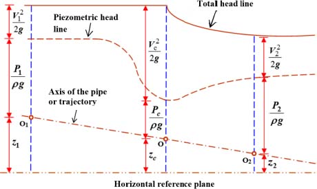
Figure 2.17. Progression of the load line and the piezometric line through a sharply narrowing segment. For a color version of this figure, see www.iste.co.uk/sadchemloul/mechanics.zip
At the level of the contracted section of the vein, the speed can reach its maximum value, while the pressure reaches its minimum value. It is therefore necessary for the absolute pressure in this section to be greater than the vapor tension of the liquid, so that the phenomenon of cavitation can be avoided.
2.6.10. Exercise 22: capillary tube
A capillary tube with radius r is submerged in a liquid of density ρ. Determine the relationship giving the height of the rise of the liquid in the capillary tube h and taking into account the surface tension σ of the liquid and the gravitational acceleration g.
2.6.10.1. Solution
The expression of the height of the rise is h = f(r, ρ,σ,g).
The number of physical quantities is n = 5, and has as its dimensions:
The number of fundamental quantities is k = 3 and the number of terms in π is n – k = 2.
If ρ, g and r are taken as chosen or repeated quantities, the terms in π are written as:
The dimension of the term π1 gives us:

and therefore ![]() .
.
The dimension of the term π2 gives us:
and therefore ![]() .
.
The terms verify the relationship  :
:
The expression of the height of the rise is:
with K as a constant.
COMMENT 2.25.– The height of rise is given by Jurin’s law20:
with θ being the angle of contact between the liquid and the tube wall, also called the juncture angle (see Figure 2.18).
When immersing a glass capillary tube in a wetting liquid, such as water (see Figure 2.18), the liquid rises relative to the level of the open surface area of the container. The concave meniscus forms an angle ![]() with the tube wall, and in the case of water θ = 0.
with the tube wall, and in the case of water θ = 0.
Because of this, it appears that a force exists that defies gravity: when we put the capillary tube in place, a curved surface forms, and in this case, Laplace’s law21 dictates a difference in pressure between the liquid and the air. Thus, we see a decrease in pressure at the convex level of the meniscus. To compensate for this reduction in pressure, the liquid sees a rise in height h, caused by a hydrostatic pressure that is greater than atmospheric pressure (P > Patm).
When the liquid does not dampen the walls of the capillary tube, that is, ![]() , a capillary depression is observed (see Figure 2.19). This capillary depression is used in mercury porosimetry. This is a technique that allows the size distribution of pores to be determined. The principle of this is based on the fact that in order for mercury to penetrate the pores of a solid, it is necessary to apply a pressure so great that the pore size is reduced.
, a capillary depression is observed (see Figure 2.19). This capillary depression is used in mercury porosimetry. This is a technique that allows the size distribution of pores to be determined. The principle of this is based on the fact that in order for mercury to penetrate the pores of a solid, it is necessary to apply a pressure so great that the pore size is reduced.

Figure 2.18. Capillary rise in the case of water that dampens the solid from which the capillary tube is created. For a color version of this figure, see www.iste.co.uk/sadchemloul/mechanics.zip
Figure 2.19. Capillary depression in the case of mercury that does not dampen the solid from which the capillary tube is made. For a color version of this figure, see www.iste.co.uk/sadchemloul/mechanics.zip
2.6.11. Exercise 23: deformation of a bubble
A bubble ascending in a fluid can remain spherical or be deformed by flattening its upper face. We may observe that the faster the bubbles move relative to the liquid, the less stable they become. Find a threshold value on a non-dimensional number above which the bubble becomes distorted. The deformation δb of the bubble depends on its radius R, its rate of ascent V, the surface tension of the fluid σ and its density ρ.
2.6.11.1. Solution
The deformation δb of the bubble is given by σb = f(R,σ,V,ρ).
The number of physical quantities is n = 5, having as their dimensions:
The number of fundamental quantities is n – k = 3 and therefore there are two terms in π.
Considering that σ, R, and ρ are chosen or repeated quantities, the terms π are written as:
The dimensions of this term π1 gives us:
And therefore:
This result is clear, because δb and R have the same dimension.
The dimensions of this term π2 gives us:
And therefore:
The terms verify the relationship:
COMMENT 2.26.– The relative deformation of the bubble depends solely on the non-dimensional term π2. The square of this term represents the Weber number. This number measures the ratio of the kinetic energy of the fluid to the energy of the bubble’s distortion. In practice, the deformation of the bubble occurs beyond a critical value of the Weber number.
Small Bond Bo numbers are found in spherical bubbles. Their ability to be distorted increases with the Bond number.
For small capillary numbers, the forces of surface tension dominate. When the capillary number is zero, the deformation of a spherical bubble is zero. The variation of the shape of the bubbles on the basis of their volume depends on the level of viscosity. In this sense, the characterization of the different shapes of the bubbles is carried out by making a distinction between water and low viscosity Newtonian fluids as compared to high viscosity Newtonian fluids.
In viscous Newtonian fluids, bubbles pass through known shapes: spherical and then ellipsoid with vertically impacted revolutions, in which the back part of the bubble is flattened until it takes on a spherical, helmet-like shape for larger volumes.
For a Newtonian fluid, regardless of its size, the bubbles do not have a tail, but after reaching a certain volume, they are given a parachute-like shape (see Figure 2.20), as a depression forms at the back of the bubble.
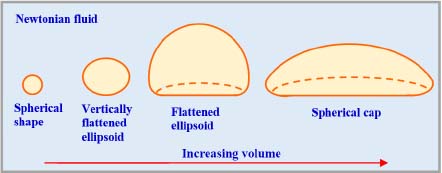
Figure 2.20. Generic form of bubbles in a Newtonian fluid. For a color version of this figure, see www.iste.co.uk/sadchemloul/mechanics.zip
2.6.12. Exercise 24: laminar dynamic boundary layer on a flat plate
Here, we will consider the laminar flow along a flat plate. The thickness of the dynamic boundary layer δ increases with the distance x at the bottom of the plate, and it also depends on the speed of the free flow U∞, the dynamic viscosity of the fluid μ and the fluid’s density ρ. Determine the expression of the dynamic boundary layer thickness δ.
2.6.12.1. Solution
The expression of the dynamic boundary layer thickness is:
The number of physical quantities is n = 5, and has as its dimensions
The number of fundamental quantities is k = 2, and therefore there are two terms in π.
Considering that ρ, U∞ and x are chosen or repeated quantities, the terms π are written as:

The dimension of the term π1 gives us:

and so ![]() , ratio between the thickness δ of the boundary layer and abscissa x where it is determined.
, ratio between the thickness δ of the boundary layer and abscissa x where it is determined.
The dimension of the term π2 gives us:

And thus ![]() is the inverse of the Reynolds number according to the length of the flat plate, which is:
is the inverse of the Reynolds number according to the length of the flat plate, which is:
Dimensional analysis makes it possible to write the following:
COMMENT 2.27.– The simplest example of an external flow is that of a fluid under a pressure P∞ which arrives at a uniform velocity U∞ parallel to a flat wall (see Figure 2.21).

Figure 2.21. Laminar dynamic boundary layer on a flat wall. For a color version of this figure, see www.iste.co.uk/sadchemloul/mechanics.zip
When the fluid is in contact with the wall, the flow is divided into two regions:
- – a region near the wall where a velocity gradient is established due to viscous forces: the particle-particle friction, and the particle-wall friction. In this region, the viscous forces are very large with respect to the inertia forces. The closer to the wall, the more the fluid is slowed, and the speed is cancelled out entirely along the surface of the wall (on the condition of adhesion to the wall). This region is known as the dynamic boundary layer;
- – a region far from the wall where the velocity gradient is zero and the forces of inertia are greater than the viscous forces. This region is also referred to as healthy flow or Euler flow22.
The dynamic boundary layer is referred to as laminar when the Reynolds number is such that Rex < 105.
The thickness of the boundary layer δ(x) is conventionally defined by:
NOTE 2.9.– In order to determine the coefficient of friction due to the flow of the fluid on the wall, it is necessary to determine the velocity profile u(y). This is given either by the exact solution, known as the “Blasius” solution, or by approximate solutions.
The following table provides a comparison between the approximate solutions and the exact solution, with δd being the displacement thickness of the boundary layer, δqm the thickness of the quantity of movement, Hf the shape factor that allows it to be determined whether or not the boundary layer will detach from the wall, the local coefficient of friction Cf, the overall coefficient of friction Cf, and RL the Reynolds number calculated over the entire length of the flat wall.
Table 2.6. Comparison between the exact solution and the approximate solutions in the case of a laminar dynamic boundary layer
| Profile |
|||
|---|---|---|---|
| Exact Solution | 5 | 1.721 | 0.664 |
| 3.464 | 1.732 | 0.577 | |
 |
5.48 | 1.83 | 0.730 |
 |
4.64 | 1.74 | 0.646 |
 |
5.84 | 1.752 | 0.686 |
| 1.741 | 1.741 | 0.654 | |
| Profile |
|||
| Exact Solution | 2.59 | 0.664 | 1.328 |
| 3.00 | 0.577 | 1.155 | |
|
2.50 | 0.730 | 1.460 |
|
2.70 | 0.646 | 1.292 |
|
2.55 | 0.686 | 1.372 |
| 2.66 | 0.654 | 1.310 |
COMMENT 2.28.– In the case of Rex > 105, the dynamic boundary layer is turbulent (see Figure 2.22). The speed profile grows much more quickly with greater distance from the wall, and as a result, turbulent friction is much higher than laminar friction. Thus, the turbulent boundary layer is much more resistant to adverse pressure gradients, so it is more difficult to separate. In this turbulent boundary layer, two regions can be identified.
- 1) The internal region. In this region, the velocity profile in the turbulent boundary layer is in a non-dimensional form u+= f(y+). This region is formed by two zones (see Figure 2.23).
Viscous sub-layer Rex < 5 or 10: immediately next to the wall, the term laminar friction is dominant, as the average velocities and velocity fluctuations tend toward zero along the wall. The scale of speed that characterizes this zone is the speed of friction. The velocity profile is determined from the local mean velocity
 , the wall stress τp, the density ρ, and the dynamic viscosity μ of the fluid, and the perpendicular distance y to the wall.
The expression of the local average speed is
 .
.The number of physical quantities is n = 5, and has as its dimensions:

The number of fundamental quantities is k = 3. Thus, there are two terms in π.
Considering that τp, y and ρ are chosen or repeated quantities, the terms π are written as:
The dimension of the terms in π gives the following expressions:

The term
 is called the “friction velocity” because it has the same dimension as a velocity and is determined from the stress along the wall (friction). The term π1 is generally written as
  . The term π2 has no dimension and represents the inverse of the Reynolds number, but a dimensional analysis allows us to write:
The two terms in π confirm the relationship:

The form of the function F1 depends on the flow behavior.
For y+ < 1, we have u+ = y+.
- – Buffer zone 5 < y+ < 30 : the connection of the linear law that is valid in the viscous sublayer and the logarithmic profile that is valid in the upper part of the inner layer occurs gradually in a buffer region.
- – Logarithmic zone (barrier law) 30 < y+ < 500: the friction between the threads of the flow primarily occur because of turbulent agitation, and the average local velocity is given by:
- 2) The external region. In this region, there are two zones:
- – Velocity deficit zone y+ > 500: as we leave the viscous sub-layer, the term of turbulent friction gradually becomes predominant with respect to laminar friction, such that as we approach the edge of the boundary layer, the laminar friction becomes negligible. The difference between the average velocity in this area and the outer velocity U∞ is on the order of magnitude of the friction velocity uf:

- – The wake zone, where movements are very disjointed. This is an important cause of the dissipation of energy. It defines the profile of velocities through a completely empirical law:
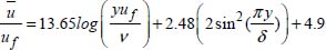
- – Velocity deficit zone y+ > 500: as we leave the viscous sub-layer, the term of turbulent friction gradually becomes predominant with respect to laminar friction, such that as we approach the edge of the boundary layer, the laminar friction becomes negligible. The difference between the average velocity

Figure 2.22. Velocity profile through the turbulent boundary layer of a flat plate. For a color version of this figure, see www.iste.co.uk/sadchemloul/mechanics.zip
2.6.13. Exercise 25: power of a stirrer
Determine the power p transmitted by a stirrer to a liquid of density ρ. The stirrer of diameter D spins at the rotational speed N.
2.6.13.1. Solution
The power transmitted by the stirrer to the liquid is given by the relationship p = f(ρ, N,D).
The number of physical quantities is n = 5, and has as its dimensions:
The number of fundamental quantities is n = 3, and therefore there is one term in π. Considering that D, ρ and N are chosen or repeated quantities, the terms π are written as π = DαρβNγp.
The dimension of the term π allows us to obtain:
The term π is written as ![]() .
.
There is only one term in π to characterize the problem, it is not a function of any other, it is necessarily constant (π = constant = K), and the relationship of the power is written as p = KρN3D5.

Figure 2.23. Scheme of a stirrer for liquids. For a color version of this figure, see www.iste.co.uk/sadchemloul/mechanics.zip
COMMENT 2.29.– The power p transferred by a stirrer to a liquid depends on the flow scheme:
- – in a turbulent regime (
 ), the power consumed by the stirring within this turbulent regime is p = (C – Co)ω, with μ being the dynamic viscosity of the liquid, C the torque transferred to the liquid, Co the torque while not subjected to a load (in the air) and N the rotating speed of the stirrer;
 - – for the turbulent regime the power number
 characterizing the energy consumption is a constant for a given agitator tank. The constant K therefore represents the power number;
 - – in the laminar scheme (Re < 10) the product Np. Re is constant.
Stirring is achieved by putting the liquid phase into movement. If the mass is made up of several components, the stirring tends to homogenize the mass in contact with the reagents, so that they react more efficiently. Most of the stirring and mixing operations are carried out by means of a tilting stirrer that rotates around a shaft placed in a vessel, which is generally cylindrical in shape. If no stirring is done, the mixture follows Fick’s law23 (molecular diffusion).
The role of the stirrer is to cause greater movement of the fluid, and therefore the agitation due to forced convection. To accomplish this, different types of stirrers have been devised, each of which has a design adapted to a given application.
There are two main classes of agitation propellers, following the movement of fluids generated in the tank relative to the axis of rotation of the mobile (see Figure 2.24):
- – axial flow mobiles, which create a flow of fluid in the tank from the top to the bottom;
- – radial flow mobiles that create radial flow perpendicular to the rotation axis.
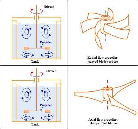
Figure 2.24. Example of axial and radial flow propellers. For a color version of this figure, see www.iste.co.uk/sadchemloul/mechanics.zip
- 1 John William Strutt, better known by his title, Lord Rayleigh, was an English physicist (1842-1919) who studied several branches of physics and mechanics (acoustics, optics, electrodynamics, electromagnetism, fluid viscosity, photography).
- 2 Aime Vaschy, born on April 9, 1857, in Thones (France) and living until November 25, 1899, was a French telegraph engineer and mathematician. Edgar Buckingham, born on July 8, 1867, in Philadelphia and living until April 29, 1940, was a physicist.
- 3 Osborne Reynolds, born on August 23, 1842, in Belfast (Northern Ireland) and who lived until February 12, 1912, was an engineer and physicist who made important contributions to hydrodynamics and to fluid dynamics, most notably the creation of the Reynolds number in 1883.
- 4 William Froude, born November 28, 1810, in Devon (England) and lived until 1879, was an engineer, hydrodynamics specialist, and naval architect.
- 5 Rheology (which derives from the Greek word rheo, meaning “flow”, and logos, referring to “study”) is the study of the deformation and flow of matter under the effect of applied stress. The word rheology was first used in 1928 by Eugene Cook Bingham (born on December 8, 1878, in Vermont (United States), and who lived until November 6, 1945); he was a professor at Lehigh University in the United States.
- 6 Moritz Weber, born on July 18, 1871, in Leipzig (Germany), and who lived until June 1o, 1951, was a fluid dynamics engineer.
- 7 Ernst Mach, born on February 18, 1838, in Chiltlitz-turas (Austria) and who lived until February 19, 1916, was a physicist and philosopher.
- 8 Henry Philibert Gaspard Darcy, born on June 10, 1803, in Dijon (France), and who lived until January 2, 1858, was a hydraulicist. Julius Ludwig Weisbach, born on August 10, 1806, in Mittelschmiedeberg (Germany), and who lived until February 24, 1871, was a mathematician and engineer.
- 9 Lewis Ferry Moody, born on January 5, 1880, in Philadelphia and who lived until February 21, 1953, was an engineer and professor, best known for devising the Moody chart.
- 10 Jean-Léonard-Marie Poiseuille, born on April 22, 1797, in Paris and who lived until December 26, 1869, was a physicist and doctor who graduated from the École polytechnique (France’s Polytechnic University).
- 11 Paul Richard Heinrich Blasius, born on August 9, 1883 in Paris, and who lived until April 24, 1970, was a French physicist who worked on fluid dynamics. He was one of the first students of Ludwig Prandtl.
- 12 Ludwig Prandtl, born on February 4, 1875, in Freising, Germany, and who lived until August 15, 1953, was an engineer and physicist. Ivan Nikuradse, born on November 20, 1894, in Samtredia, in the country of Georgia, and who died on July 18, 1979, was an engineer and physicist.
- 13 Theodore Von Kármán, born on May 11, 1881, in Budapest (Hungary), and who lived until May 6, 1963, was an engineer and physicist who specialized in aeronautics.
- 14 Cyril Frank Colebrook, born on July 26, 1910, in Swansea, Wales, and who lived until January 12, 1997, was a physicist. This relationship very correctly reflects the behaviors of industrial pipes, for which the functionality schemes often correspond to the domain of transition.
- 15 George Gabriel Stokes, born on August 13, 1819, in Skreen (Ireland), and who lived until February 1, 1903, was a mathematician and physicist. He made his biggest contributions in the areas of fluid mechanics, optics and geodesy. The movement of a Newtonian fluid is referred to as Navier-Stokes equations, which are the work of two scientists in the 19th Century: the mathematician and bridge engineer Henri Navier, who introduced first the notion of viscosity in the Euler equations in 1823, and the physicist George Gabriel Stokes who provided the definitive form of the equation of conservation of the quantity of movement in 1845.
- 16 Archimedes of Syracuse, born in Syracuse (Italy) around 287 B.C. and who lived until 212 B.C., was a physicist, mathematician and engineer.
- 17 This result had been found by Rayleigh and published in the journal Nature in 1915 in an article named “The Principle of Similitude”, vol. no. 95, pp. 66–68.
- 18 Jean Baptiste Charles Joseph Belanger, born on April 4, 1790, and who lived until May 8, 1874, was a mathematician who worked in the field of hydraulics and hydrodynamics.
- 19 Barré de Saint Venant, born on August 23, 1797, in the Château de Fortoiseau, in Villiersen-Bière (Seine-et-Marne, France) and who lived until January 6, 1886, was an engineer, physicist, and mathematician.
- 20 James Jurin, born on December 15, 1684, and living until March 29, 1750, was an English doctor and physicist who left a legacy of pioneering works on capillary actions and epidemiology (inoculation).
- 21 Pierre-Simon de Laplace, born on March 23, 1749, in Beaumont-en-Auge (France) and who lived until March 5, 1827, was a mathematician, astronomer, physicist and political figure.
- 22 Leonhard Euler, born on April 15, 1707, in Basel (Switzerland), and who lived until September 18, 1783, was a mathematician and physician.
- 23 Adolf Eugene Fick, born on September 3, 1829, in Kassel (Germany), and living until August 21, 1901, was a physiologist. In 1851, he became a doctor of medicine. In 1855, he introduced two phenomenological laws addressing the diffusion of matter, known as Fick’s laws.