Chapter 9 Object Classification in a Distributed Environment

Object classification is the process of providing some level of identification of an object, whether it is at a very specific level or at a general level. In a defense or security environment, such classes can range from distinguishing people from vehicles, a type of vehicle, or in more specific cases a particular object or entity, even to the “serial number.” Of course, another fundamental classification for such purposes is the traditional friend-foe-neutral-unknown class categories that are used in developing action-taking policies and decisions. The concept of identity is an interesting one and is nonmetric in that there is no generalized or unified scale of units by which we “measure” the identity of an object. The nonmetric nature of the identity of an object has motivated the formation of several alternative approaches to the representation, quantification, and manipulation of uncertainty in identity. Statistical methods, fuzzy set (possibilistic), and neural network methods are some of the popular methods that have been applied to this problem but two statistically based techniques remain the most popular: Bayesian methods and Dempster–Shafer methods. For decentralized/distributed applications, these two approaches have the attractive features that they are both commutative and associative; so results are independent of the order in which data are received and processed.

Dempster–Shafer methods (Al-Ani and Deriche 2002) were largely developed to overcome the apparent inability of the Bayesian formalism to adequately deal with “unknown” classes, as opposed to an estimated degree of ignorance attempted in Dempster–Shafer. However, achieving this feature is usually at the expense of computationally more intensive algorithms. The distributed classification problem raises a number of architectural problems, and two key challenges are (1) how to connect all the sensors and processing nodes together (these are organizational and architecture issues) and (2) how to fuse the data for estimates generated by the nodal operations (this is a data fusion algorithm design issue).

By and large, an object’s class is discerned by an examination of its features or attributes where we distinguish a feature as an observed characteristic of an object and an attribute as an inherent characteristic. As regards information fusion processing, automated classification techniques are placed in the “Level 1” category of the JDL data fusion process model where, in conjunction with tracking and kinematic estimation operations, they help to answer two fundamental questions “Where is it?” and “What is it?” One can quickly get philosophical about the concept of class and identity, and there are various works the reader can examine to explore these viewpoints, such as Zalta (2012) and Hartshorne et al. (1931–1958). As just mentioned, identity and/or class membership is determined from features and attributes (F&A henceforth) by some type of pattern recognition process that is able to assign a label to the object according to the F&A estimates and perhaps some ontology or taxonomy of object types and classes. Assigning an identity label is not an absolute process; classification of an object may, for example, be context-dependent (e.g., whether an object is in the class “large” or not may be dependent on its surroundings).

The structure of this chapter is as follows: in Section 9.2 we provide a limited overview of object classification approaches, in Section 9.3 a summary of classification architectures is provided. Section 9.4 addresses distributed object classification issues, Section 9.5 discusses classifier fusion, and Section 9.6 provides an extended discussion on distributed Bayesian classification and performance evaluation, as the Bayes formalism remains a central methodology for many classification problems.

9.2 OVERVIEW OF OBJECT CLASSIFICATION APPROACHES

The data and information fusion community, as well as the remote sensing community, have a long history of research in exploring and developing automated methods for estimating an object’s class from available observational data on F&A, which is the fundamental goal of object/entity classification. In a broad sense, the basic processing steps for classification involve sensor-dependent preprocessing that in the multisensor fusion case includes common referencing or alignment (for imaging sensors often used for classification operations, this is typically called co-registration), F&A extraction, F&A association, and class-estimation. There are many complexities in attempting to automate this process since the mapping between F&A and the ability to assign an object label is a very complex relationship, which is complicated by the usual observation errors and, in the military domain, by efforts of the adversary to incorporate decoys and deception techniques to create ambiguous F&A characteristics. In the military domain, these works have usually come under the labels of “automated” or “assisted” or “aided” target recognition or “ATR” methods, also non-cooperative target recognition (NCTR) methods, and there have been many conferences and published works on these topics. We find no very recent open-source publications explicitly directed to state-of-the-art assessments of ATR/NCTR technology but some state-of-the-art and survey literature does exist, such as those by Bhanu (1986), Roth (1990), Cohen (1991), Novak (2000), and Murphy and Taylor(2002), but nothing very recent in the timeframe of this book. The most central source for publications on ATR and the broader topic of object classification are the SPIE defense conferences held annually for a number of years, and the interested reader is referred to this source for additional information. On the other hand, there are some more recent works that review the broader domain of classification methods as a general problem. Still, no overarching state-of-the-art work has been done, but there are various survey papers directed to certain classes of methods.

One way to summarize alternative approaches to classification is provided by bisecting the methods into the “discriminative” and “generative” types; a number of recent references address this topic, such as Ng and Jordan (2002). Generative classification methods assume some functional form for the conditional relation between the F&A data and the class labeling, and estimate the parameters of these functions directly from truthed training data. An example is Naïve Bayes where the generative approach takes the form of the relation as P(Features|Class Label), and the model of the prior existence of a class label as P(Class Label); in typical notation these are P(X|Y) and P(Y). Additional generative techniques include model-based recognition, Gaussian mixture densities, and Bayesian networks. Discriminative classifiers are methods constructed to directly learn the relation P(Class Label|F&A Data), or directly learn P(Y|X). An example often cited in the literature is logistic regression but other methods include neural networks, various discriminant classifiers, and support vector machines.

Montillo (2010) asserts the advantages and disadvantages of the generative approach in Table 9.1. And similarly, the trade-offs are also asserted by Montillo for the discriminative approaches in Table 9.2.

The interested reader is also directed to the various citations for both the ATR/NCTR literature that, while somewhat dated, still gives some valuable insight, and into the generative, discriminative comparative literature for a somewhat more modern view.

TABLE 9.1
Features of Generative Approaches to Classification

Advantages	Disadvantages
Ability to introduce prior knowledge	Marred by generic optimization criteria
Do not require large training sets	Potentially wasteful modeling
Generation of synthetic inputs	Reliant on domain expertise
	Do not scale well to large number of classes

Source: Adapted from Montillo, A., Generative versus discriminative modeling frameworks, Lecture at Temple University, http://www.albertmontillo.com/lectures,presentations/Generative%20vs%20Discriminative.pdf, 2010.

TABLE 9.2
Features of Discriminative Approaches to Classification

Advantages	Disadvantages
Fast prediction speed	Task specific
Potentially more accurate prediction	Long training time
	Do not easily handle compositionality

It is beyond the scope of this chapter to provide further detail on these state-of-the-art and survey remarks, nor a tutorial-type overview of this extensive field; for the most up-to-date open-source information, we again suggest the SPIE conference literature, the IEEE Pattern Analysis and Machine Intelligence Transactions, and for tutorials the interested reader is referred to such books as those by Tait (2005), Sadjadi and Javidi (2007), or Nebabin (1994).

9.3 ARCHITECTURAL OPTIONS FOR OBJECT CLASSIFICATION

To better understand the content of this chapter, we offer some perspectives on the structural design of an object classification process as determined by multiple observational data. A notional set of architectural configurations for object classification processing is shown in Figure 9.1.

In a distributed context, it could be for example that each sensor-specific processing thread is a node in a network, and the Declaration Fusion process is occurring at a receiving node that collects each sensor-specific declaration of class. There are many possible variations of the different ways a distributed classification process may operate but this figure should be adequate for our purpose. We characterize the process as involving multiple sensor systems (S1, S2) that each generates (imperfect) observational data. Three alternative processing schemes are shown: a measurement-based approach, a feature-based approach, and a decision-based approach. As mentioned earlier, the processes shown can happen within a node in a network (local/single-node-multisensor fusion) or they can represent internodal, distributed operations where sensor-specific operations at one node are then sent, via the network, to another (receiving node) where the multisensor fusion would take place. In either case, these are the following characteristics of each operation:

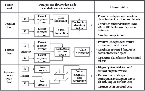
FIGURE 9.1 Notional multisensor object classification process options.

• The measurement-based approach ideally would use combined raw sensor data at the measurement (pre-feature) level to form information-rich features and attributes that would then provide the evidential foundation for a classification/recognition/identification algorithm. Note that in the distributed case this involves sending raw measurement data across the network, often considered prohibitive due to bandwidth limitations.

• The feature-based approach involves sensor-specific computation of available features, then a combining/fusing of the features as the evidential basis for classification. In the distributed case, the features would be communicated to other nodes.

• The decision-based approach has the sensor-specific processing proceeding to the declaration/decision level, after which the decisions are fused. Decisions can be sent over the network using lower bandwidth links or by consuming small amounts of any given bandwidth.

Note too that for measurement- and feature-based approaches, there is a requirement to co-register or align the data (in the “common referencing” function of a fusion process) before the combining operations take place. Registration requirements are most stringent for the most detailed type of data, so that the highest precision in registration is needed for the measurement-based operations.

In the case of distributed object classification, clearly what happens regarding fusion operations at any receiving node is dependent on what has been transmitted; of course, it is possible that mixtures of types of data may also arrive at the receiving node. For any distributed environment, it should be noted that any node can only fuse two things: those data that it “owns” (typically called “organic” data), and data that come to it somehow over the network. Thus, in the distributed case, a crucial design issue is the specification of what we call here “information-sharing strategies” that govern who sends what to whom, how often, in what format, etc.; this issue is crucial but outside the scope of this chapter.

9.4 ISSUES IN DISTRIBUTED OBJECT CLASSIFICATION

Distributed target tracking and classification have become a popular area of research because of the proliferation of sensors (Brooks et al. 2003, Kotecha et al. 2005). The issues related to distributed object classification are analogous to the issues associated with distributed tracking (Liggins et al. 1997), which include the issue of correlated data and decisions and the associated effects on the fused result. As in any fusion process, consideration of the common referencing, data association, and state estimation functions and how they might be affected by the peculiarities of the distributed environment needs to be carried out. In large networks, it is typical that any given node has limited knowledge of the functions and capabilities of the other nodes in the network; it is often assumed that any given node only knows specific information about its neighboring nodes but not distant nodes. This situation imputes the requirement for sending/transmitting nodes to append metadata to their messages to provide adequate information to receiving nodes such as to allow proper processing of the information in the received messages. This metadata has come to be called “pedigree” information by the fusion community, and one definition of pedigree is that it is information needed by a receiving node such as to assure the mathematical or formal integrity of whatever operation it applies to the received data, although the extent of the pedigree content may include yet other information.

Later we provide a brief description and a simple diagrammatic summary of some typical issues in distributed classification operations. Four cases will be described: “explicit” double-counting, “implicit” double-counting (statistically dependent case), hard declarations resulting from legacy systems, and mixed uncertainty representations; many other issues are possible in the distributed object ID case but these are some typical examples. It should also be noted that combinations of these cases could arise in any practical environment. Note also that none of these case models depict the further ramifications of feedback from fusion nodes to sender/contributor nodes; such feedback adds another layer of complexity to the pedigree operations. The later sections of this chapter address some of the issues raised herein in some detail.

9.4.1 EXPLICIT DOUBLE-COUNTING

One concern in such environments, if the connectivity structure and message-handling protocols are not specified in a very detailed way, is about the problem of “double-counting,” wherein information in sent-messages appear to return to the original sending node as newly received messages with seemingly new, complementary information. If such messages had a “lineage” or “pedigree” tag describing their processing history, the recipient could understand that the message was indeed the same as what it had sent out earlier. This type of double-counting (also known as “data incest,” “rumor propagation,” and “self-intoxication”) can be called “explicit,” in that it is literally the result of reception of a previously sent and processed message, simply returning to the sender. This process is shown in Figure 9.2.

9.4.2 IMPLICIT DOUBLE-COUNTING (STATISTICALLY DEPENDENT)

A fundamental concern, due to the nature of the statistical mathematics often involved in classifier or ID fusion operations, is the issue of statistical independence (or dependence) of the communicated or shared information. The major issue here revolves about the complexity of the required modeling and mathematics if the information to be fused is statistically dependent, and the resulting errors in processing if independence assumptions are violated. This problem can be called one of “implicit” double-counting, in that the redundant portion of the fused information is an idiosyncrasy of the sensing and classification operations involved and are hidden, in effect. Figure 9.3 shows the idea.

In this case, the local/sending node uses two sensor-specific classifiers, and the performance of the individual classifiers is quantified using confusion matrices, resulting in the statistical quantification as shown (Prob(ID|Features)), which is sent to the fusion node along with the declarations. Note that the sensors provide a common feature/attribute F1 that is used by both sensor-specific classifiers, resulting in the individual classifier outputs being correlated. The receiving fusion node operates on the probabilities in a Bayesian way to develop the fused estimate but may erroneously assume independence of the received soft declarations, and thereby double-count the effects of Feature F1, upon which both individual declarations are based. Pedigree tags would signify the features upon which the decisions are based.

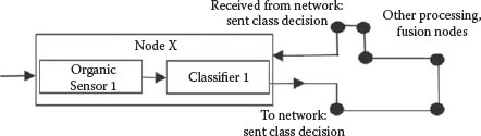
FIGURE 9.2 Explicit double-counting.

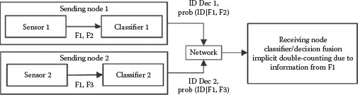
FIGURE 9.3 Implicit double-counting.

9.4.3 LEGACY SYSTEMS WITH HARD DECLARATIONS

Further, if the distributed network includes nodes that are “legacy” systems (i.e., previously built components constructed without forethought of embedding them in a fusion network), it is likely that either (1) ID classifiers will be “hard” classifiers, producing ID declarations without confidence measures (“votes” in essence) or (2) the confidence measures employed will not be consistent with other confidence measures employed by other network classifiers. In the first case, fusion can only occur with a type of voting strategy and likely without formal consideration of statistical independence aspects and any pedigree-related processing regarding this issue. Improvements can be made to this fusion approach if the rank-order of the ID declarations is also available (see Figure 9.4). In the second case, some type of uncertainty-measure-transformations need to be made to normalize the uncertainty representation into some common framework for a fusion operation.

In this representative situation, existing legacy sensor-classifier systems produce “hard” ID declarations, i.e., without qualification—these are “votes” in effect. Fusion methods can include simple voting-based strategies (majority, plurality, etc.), which may overtly ignore possible correlations as shown (common ID feature F1 as in the previous example). However, it is possible to develop voting schemes that derive from trained data, which, if the training data are truly representative, may empirically account for the effects of correlated parameters to some degree. Here again the pedigree tag would include the parameters upon which the local-node/sent IDs are based.

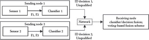
FIGURE 9.4 Legacy systems with hard decisions.

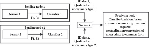
FIGURE 9.5 Classifiers with mixed uncertainty representations.

9.4.4 MIXED UNCERTAINTY REPRESENTATIONS

In this case, we have classifiers whose performance is quantified using different uncertainty types, e.g., probabilistic and evidential (Figure 9.5 just shows uncertainty types 1 and 2). The confounding effects of correlated observations may still exist. The fusion process is dependent on which uncertainty form is normalized, e.g., if the evidential form is transformed to the probabilistic form, then a Bayesian fusion process could be employed. Here, the pedigree tag must also include the type of uncertainty employed by each classifier evaluation scheme. As will be discussed later, it is also very important that the nature of such statistical or other transformations is well-understood and properly included in the fusion scheme.

As noted earlier, it is possible that real-world systems and networks may employ several sensor-classifier systems as input or in some shared/distributed framework, and combinations of the aforementioned cases could result, adding to the overall complexity of the fusion operations at some receiving node. Depending on how the overall system is architected, it may be necessary to have the pedigree tags include all possible effects, even if some particular tag elements are null.

9.5 CLASSIFIER FUSION

Here, we provide a brief overview of classifier combining methods drawn from some often-cited works that contain most of the details (e.g., Ho et al. 1994, Kittler et al. 1998, Kuncheva 2002). We begin with a taxonomic categorization as asserted in Ruta and Gabrys (2000), and then provide a point-by-point commentary on the most traditional classifier combining techniques. There are two main motivations for combining classifier results: efficiency and accuracy. Efficiencies can be achieved in multiclassifier systems by tuning the system to use the most appropriate, least computationally intensive classifier at any given moment in an application. Accuracy improvements can be realized in multiclassifier systems by combining methods that employ different sensor data and/or features, or have nuanced algorithmic features that offer some special benefit; the broad idea here is exploitation of diversity although diversity in classification can be a controversial topic. In a distributed object classification system, the classifier results from multiple nodes also have to be combined.

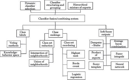
FIGURE 9.6 A taxonomy of classifier fusion techniques. (Adapted from Ruta, D. and Gabrys, B., Comput. Inf. Syst., 7, 1, 2000.)

9.5.1 TAXONOMY OF CLASSIFIER FUSION METHODS

One taxonomy of classifier fusion methods is offered in Ruta and Gabrys (2000) and is shown in Figure 9.6.

As noted earlier, the choice of fusion approach (also often called “classifier combining” in the literature) is dependent on the type of information being shared. Here, when only hard (unqualified) labels or decisions are provided, a typical approach to fusion is via voting methods. (It should be noted that there are many different strategies for voting, well beyond the usual plurality, majority-based techniques [see Llinas et al. 1998].) Much of the fusion literature has addressed the cases involving soft or fuzzy outputs as shown in Figure 9.6, where the class labels provided by any classifier are quantitatively qualified, for example with the conditional probabilities that come from the testing/calibration of that classifier, as just described. When such information is available, the fusion or combining processes can exploit the qualifier (probabilistic) information in statistical-type operations.

9.5.2 COMBINING CLASSIFIERS

The options available for classifier combining are influenced by various factors. If, for example, only “labels” are available,^* various voting techniques can be employed; see Llinas et al. (1998) for an overview of voting-based combining methods for either label declarations or hard declarations. If continuous outputs like posterior probabilities are supplied (these are called “soft” declarations), then a variety of combining strategies are possible, again assuming a consistent, probabilistically based uncertainty representational form is used by all contributing classifiers (recall Section 9.4.4). For other than probabilistic but consistent representational forms of uncertainty such as fuzzy membership values, possibilistic forms, and evidential forms, the algebra of each method can be used in the classifier combining process (e.g., the Dempster Rule of Combination in the evidential case). Of course, all of these comments presume that the class-context of each contributing classifier is semantically consistent, otherwise some type of semantic, and associated mathematical transforms would need to be made. For example, it makes no sense to combine posterior probabilities if they are probabilities about inconsistent classes or class-types.

Kittler et al. (1998) describes what he says are two basic classifier-combining scenarios: one in which all classifiers are provided a common data set (one could call this an “algorithm-combining” approach, since the effects on the combined result are the consequence of distinctions in the various classifier algorithms), and an approach where each classifier is receiving unique data from disparate sources (as in a distributed system); Kittler’s often-cited paper focuses on the latter. This paper describes the commonly used classifier combination schemes such as the product rule, sum rule, min rule, max rule, median rule, and majority voting, and conducts comparative experiments that show the sum rule to outperform the others in these particular tests.

To show the flavor of these combining rules, we follow Kittler’s development for the product rule as one example; interested readers should refer to the original paper and yet other references for additional detail (e.g., Duda et al. 2001). Consider several classifier algorithms that are each provided with specific sensor measurement data and feature/attribute set. Using Kittler’s notation, let the measurement vector used by the ith classifier denoted as x_i, and each class or class-type denoted as ω_i, with prior probability given by P(ω_i). The Bayesian (the only paradigm addressed in this chapter) classification problem is to determine the class, given a measurement vector Z, which is the concatenation of the x_i, as follows:

$\begin{matrix} assign Z \to ω_{f} i f \\ P (ω_{f} | x_{1}, \dots, x_{R}) = \max_{ω_{k}} P (ω_{k} | x_{1}, \dots, x_{R}) \end{matrix}$

(9.1)

That is, the fused class label ω_f is the maximum posterior probability (MAP) solution. It should be noted that the inherent calculation of the posterior does not, in and of itself, yield a class declaration; deciding a class estimate from the posteriors is a separate, decision-making step. Strictly speaking, these calculations ideally require knowledge about the conditional probability P(x₁, …, x_R | ω_k) which would reveal the insights about inter-source dependence in (x₁, …, x_R). If we allow, as is very often done, the assumption that the sources are conditionally independent given each class, i.e.,

$P (x_{1}, \dots, x_{R} | ω_{k}) = \prod_{i = 1}^{R} P (x_{i} | ω_{k})$

(9.2)

then

$\begin{matrix} assign Z \to ω_{f} if \\ P (ω_{f}) \prod_{i = 1}^{R} P (x_{i} | ω_{f}) = \max_{ω_{k}} P (ω_{k}) \prod_{i = 1}^{R} P (x_{i} | ω_{k}) \end{matrix}$

(9.3)

Or, in terms of the individual posteriors declared by each contributing classifier,

$\begin{matrix} assign Z \to ω_{f} if \\ P^{- (R - 1)} (ω_{f}) \prod_{i = 1}^{R} P (ω_{f} | x_{i}) = \max_{ω_{k}} P^{- (R - 1)} (ω_{k}) \prod_{i = 1}^{R} P (ω_{k} | x_{i}) \end{matrix}$

(9.4)

Equation 9.4 is called the “Product Rule” for combining classifiers. It removes double-counting due to the common prior P(ω_i) but assumes conditional independence of the supporting evidence for each of the contributing Bayes classifiers. This rule is called “naïve” Bayes combination rule because in many cases there may be unmodeled statistical dependence in (x₁, …, x_R), as was discussed in Section 9.4. While strictly correct in a Bayesian sense, this rule has the vulnerability that a single bad classifier declaration having a very small posterior can inhibit an otherwise correct or appealing declaration. Other rules such as the sum rule follow similar developments but involve different assumptions (e.g., equal priors). Each of these strategies has trade-off factors regarding performance and accuracy; Kittler et al. (1998) developed an interesting analysis that explains why the sum rule seems to perform best in their experiments. Similar research is shown in the work of Kuncheva (2002) in which some six different classifier fusion strategies were examined for a simplified, two-class problem, and for which the individual-classifier error distributions were defined as either normal or uniform, and for which the individual classifiers were assumed independent. The particular fusion strategies examined were similar to some of those asserted in Kittler et al. (1998): minimum, maximum, average, median, majority vote.

9.6 OPTIMAL DISTRIBUTED BAYESIAN OBJECT CLASSIFICATION

The naïve classifier fusion approach described in Section 9.5 is easy to implement. However, it does not address the “double-counting” issues discussed in Section 9.4. This section presents an optimal distributed Bayesian object classification approach and compares its performance to the naïve fusion approach. Most of this section is from Chong and Mori (2005).

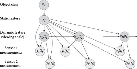
FIGURE 9.7 Bayesian network model for object classification.

Bayesian object classification uses the generative approach discussed in Section 9.2. We use the Bayesian network formalism to represent the model relating the object class to the sensor measurements. A Bayesian network (Jensen 2001, Pearl 1988) is a graphical representation of a probabilistic model. It is a directed graph where the nodes represent random variables or random vectors of interest and the directed links represent probabilistic relationships between the variables. A dynamic Bayesian network is one in which some of the nodes are indexed by time. A key feature of Bayesian networks is the explicit representation of conditional independence needed for optimal distributed object classification.

Figure 9.7 is the dynamic Bayesian network for object classification using two sensors. The variables in this network are the object class x_T, static feature x_S such as object size, dynamic feature x_D(t) (e.g., viewing angle) that varies with time, and sensor measurement y_i(t) for each sensor i.

The graph of the Bayesian network displays structural information such as the dependence among the random variables. The quantitative information for the model is represented by conditional probabilities of the random variables at the nodes given their predecessor nodes. For the network of Figure 9.7, these probabilities are as follows:

• P(x_T): prior probability of the object class.

• P(x_S|x_T): conditional probability of the static feature given the object class.

• P(x_D(t_k)|x_D(t_k−1), x_S): conditional probability of the dynamic feature x_D(t_k) at time t_k given the dynamic feature x_D(t_k−1) at time t_k−1 and the static feature x_S. If the evolution of the dynamic state does not depend on the static feature, then the conditional probability becomes P(x_D(t_k)|x_D(t_k−1)).

• P(y_i(t_k)|x_D(t_k), x_S): conditional probability of the measurement y_i(t_k) of sensor i at time t_k given the dynamic feature x_D(t_k) and the static feature x_S. This probability captures the effect of the dynamic feature on the measurement, e.g., measured size as a function of viewing angle as well as measurement error.

9.6.1 CENTRALIZED OBJECT CLASSIFICATION ALGORITHM

Suppose Y(t_k) = (y(t₁), y(t₂), …, y(t_k)) are the cumulative measurements from one or more sensors. The objective of object classification is to compute P(x_T|Y(t_k)), the probability of the object class given Y(t_k). It can be shown (see Chong and Mori [2005] for details) that this probability can be computed by the following steps:

1. Estimating dynamic and static features (x_S, x_D(t_k))

Prediction:

$P (x_{S}, x_{D} (t_{k}) | Y (t_{k - 1})) = \int P (x_{D} (t_{k}) | x_{D} (t_{k - 1}), x_{S}) P (x_{S}, x_{D} (t_{k - 1}) | Y (t_{k - 1})) d x_{D} (t_{k - 1})$

(9.5)

Update:

$P (x_{S}, x_{D} (t_{k}) | Y (t_{k})) = C^{- 1} P (y (t_{k}) | x_{D} (t_{k}), x_{S}) P (x_{S}, x_{D} (t_{k}) | Y (t_{k - 1}))$

(9.6)

2. Estimating static feature x_S

$P (x_{S} | Y (t_{k})) = \int P (x_{S}, x_{D} (t_{k}) | Y (t_{k})) d x_{D} (t_{k})$

(9.7)

3. Estimating object class x_T

$P (x_{T} | Y (t_{k})) = \int P (x_{S} | Y (t_{k})) P (x_{T} | x_{S}) d x_{S}$

(9.8)

Note that the joint estimation of the dynamic and state features is crucial since the sensor measurements depend on both features. The posterior probability of these features is updated whenever a new measurement is received. Object classification is basically a decoupled problem, with the posterior-type probability updated only when this information is needed.

Equations 9.5, 9.7, 9.8 can be used by a local fusion agent processing the measurements from a single sensor or a central fusion agent processing all sensor measurements by incorporating the appropriate sensor models. The prediction Equation 9.5 is independent of the sensor, except when different sensors observe different static features. In that case, Equation 9.5 predicts only the part of the static feature x_Si that is relevant to that sensor i.

9.6.2 DISTRIBUTED OBJECT CLASSIFICATION

The distributed object classification problem is combining estimates from the local classification agents to obtain an improved estimate of the object class. There are two tightly coupled parts of this problem. This first is determining the information sent from the local agent to the fusion agent. The second is combining the received information.

It is well known that combining the local object declarations, i.e., tank or truck, is suboptimal since the confidence in the declaration is not used. A common and better approach is to communicate the posterior-type probabilities P(x_T|Y_i) given the measurements for each sensor i and then combine the probabilities by the product rule

$P (x_{T} | Y_{1}, Y_{2}) = C^{- 1} P (x_{T} | Y_{1}) P (x_{T} | Y_{2})$

(9.9)

However, this rule is still suboptimal because the measurement sets Y₁ and Y₂ are in general not conditionally independent given the object class. This section applies the general approach for distributed estimation (Chong et al. 2012) to the distributed object classification algorithm.

9.6.2.1 Bayesian Distributed Fusion Algorithm

Let x be the state of interest, which may include the object class, as well as the static or dynamic features. Let Y₁ and Y₂ be the measurements collected by two sensors 1 and 2. Suppose the local measurement sets are conditionally independent given the state, i.e., P(Y₁, Y₂|x) = P(Y₁|x)P(Y₂|x). Then the global posterior probability can be reconstructed from the local posterior probabilities by (Chong et al. 1990)

$P (x | Y_{1}, Y_{2}) = C^{- 1} \frac{P (x | Y_{1}) P (x | Y_{2})}{P (x)}$

(9.10)

where C is a normalization constant. Note that the prior probability P(x) appears in the denominator since this common information is used to compute each local posterior probability. Equation 9.10 can also written as

$P (x | Y_{1}, Y_{2}) = C^{- 1} P (Y_{1} | x) P (x | Y_{2}) = C^{- 1} P (Y_{2} | x) P (x | Y_{1})$

(9.11)

$P (x | Y_{1}, Y_{2}) = C^{- 1} P (Y_{2} | x) P (x | Y_{1})$

by recognizing that $P (x | Y_{i}) = C_{i}^{- 1} P (Y_{i} | x) P (x)$ where C_i is a normalization constant.

For the hierarchical classification architecture, let Y_F be the set of cumulative measurements at the fusion agent F, and Y_i be the new measurements from the agent i sending the estimate. The measurement sets of the two agents are disjoint, i.e., Y_F ∩ Y_i = ϕ. Suppose the state x is chosen such that Y_F and Y_i are conditionally independent given x.

Then Equations 9.10 and 9.11 imply the fusion equations

$P (x | Y_{i}, Y_{F}) = C^{- 1} \frac{P (x | Y_{i}) P (x | Y_{F})}{P (x)}$

(9.12)

$P (x | Y_{i}, Y_{F}) = C^{- 1} P (Y_{i} | x) P (x | Y_{F})$

(9.13)

Equations 9.12 and 9.13 represent two different but equivalent approaches of communication and fusion. The first is for the local agent to send the local posterior probability P(x|Y_i) given the new measurements Y_i. The fusion agent then combines it with its posterior probability P(x|Y_F) using Equation 9.12. The second is for the local agent to send the local likelihood P(Y_i|x), which is then combined with the probability P(x|Y_F) using Equation 9.13.

A necessary condition for Equations 9.10, 9.11, 9.12, 9.13 to be optimal is the conditional independence assumption of Y₁ and Y₂. From Figure 9.7, it can be seen that choosing object class as the state will not satisfy the conditional independence condition. Thus, fusing the object class probability may be suboptimal.

9.6.2.2 Optimal Distributed Object Classification

Consider the model of Figure 9.7 and the hierarchical without feedback fusion architecture. Each local classification agent processes its sensor measurements to generate the posterior probability of a “state.” Periodically, it sends the local probability based upon the measurements received since the last communication to the high-level fusion agent. The high-level fusion agent then combines the received probabilities with its current posterior probability.

Figure 9.8 is the network of Figure 9.7 redrawn to show the measurement sets without displaying the high-level nodes x_T and x_S. At the current fusion time $t_{F + k}$ , the local fusion agent i sends the conditional probability given Y_i(t_{F + 1}, t_{F + k}) ≜ (y_i(t_{F + 1}),…, y_i(t_{F + k})), the measurements collected since the last fusion time t_F. The fusion agent then fuses this probability with its probability based upon the measurements Y_F(t₁, t_F) = ((y_i(t₁), …, y_i(t_F)); i = 1, 2).

A key problem is determining the random variable or state that satisfies the conditional independence assumption for the measurement sets so that the fusion equation can be used. The Bayesian network (Chong and Mori 2004) provides an easy way of determining this conditional independence. From Figures 9.7 and 9.8, the measurement sets Y_i(t_{F + 1}, t_{F + k}) and Y_F(t₁, t_F) are conditionally independent given x_S and the dynamic features x_D(t_{F + 1}, t_{F + k}) ≜ (x_D(t_{F + 1}), x_D(t_{F + 2}), …, x_D(t_{F + k})). However, they are not conditionally independent given x_S and the dynamic feature x_D(t_k) at a single time. Thus the state to be used for fusion is (x_S, x_D(t_{F + 1}, t_{F + k})) and the fusion process consists of the following steps:

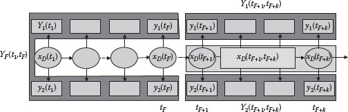
FIGURE 9.8 Conditionally independent measurements.

1. Communication by local agent. At time t_{F + k}, the local agent i sends to the high-level fusion agent the probability distribution P(x_S, x_D(t_{F + 1}, t_{F + k})|Y_i(t_{F + 1}, t_{F + k})), which can be computed by the following recursive algorithm. Let m = F + 1, n = F + 1, …, F + k − 1, x_D(t_{F + 1}, t_{F + 1}) = x_D(t_{F + 1}), and Y_i(t_{F + 1}, t_{F + 1}) = y_i(t_F+1). Then

$\begin{array}{l} P (x_{S}, x_{D} (t_{m}, t_{n + 1}) | Y_{i} (t_{m}, t_{n + 1})) \\ = C^{- 1} P (y_{i} (t_{n + 1}) | x_{S}, x_{D} (t_{n + 1})) P (x_{D} (t_{n + 1}) | x_{S}, x_{D} (t_{n})) \\ P (x_{S}, x_{D} (t_{m}, t_{n}) | Y_{i} (t_{m}, t_{n})) \end{array}$

(9.14)

Alternatively, the local agent sends the likelihood P(Y_i(t_{F + 1}, t_{F + k})|x_S, x_D(t_{F + 1}, t_{F + k})) to the high-level fusion agent. This likelihood is computed directly from the probability model

$P (Y_{i} (t_{F + 1}, t_{F + k}) | x_{S}, x_{D} (t_{F + 1}, t_{F + k})) = \prod_{m = F + 1}^{F + k} P (Y_{i} (t_{m}) | x_{s}, x_{D} (t_{m}))$

(9.15)

The prior probability P(x_S, x_D(t_{F + 1}, t_{F + k})) is given by the recursion

$\begin{array}{l} P (x_{S}, x_{D} (t_{m}, t_{n + 1})) & = P (x_{S}, x_{D} (t_{m}, t_{n}), x_{D} (t_{n + 1})) \\ = P (x_{D} (t_{n + 1}) | x_{S}, x_{D} (t_{n})) P (x_{S}, x_{D} (t_{m}, t_{n})) \end{array}$

(9.16)

2. Extrapolation by high-level agent. The high-level fusion agent computes the probability P(x_S, x_D(t_{F + 1}, t_{F + k})|Y_F(t₁, t_F)) by extrapolating P(x_S, x_D(t_F)|Y_F(t₁, t_F)) to obtain

$\begin{array}{l} P (x_{S}, x_{D} (t_{F + 1}) | Y_{F} (t_{1}, t_{F})) \\ = \int P (x_{S}, x_{D} (t_{F + 1}), x_{D} (t_{F}) | Y_{F} (t_{1}, t_{F})) d x_{D} (t_{F}) \\ = \int P (x_{D} (t_{F + 1}) | x_{D} (t_{F}), x_{S}) P (x_{S}, x_{D} (t_{F}) | Y_{F} (t_{1}, t_{F})) d x_{D} (t_{F}) \end{array}$

(9.17)

and then using the recursion

$\begin{array}{l} P (x_{S}, x_{D} (t_{F + 1}, t_{F + i + 1}) | Y_{F} (t_{1}, t_{F})) \\ = P (x_{S}, x_{D} (t_{F + 1}, t_{F + i}), x_{D} (t_{F + i + 1}) | Y_{F} (t_{1}, t_{F})) \\ = P (x_{D} (t_{F + i + 1}) | x_{S}, x_{D} (t_{F + i})) P (x_{S}, x_{D} (t_{F + 1}, t_{F + i}) | Y_{F} (t_{1}, t_{F})) \end{array}$

(9.18)

If the high-level fusion agent has fused the probability from another sensor j, then its current posterior probability P(x_S, x_D(t_{F + 1}, t_{F + k})|Y_F(t_{F + 1}, t_{F + k})) is already computed for x_D(t_{F + 1}, t_{F + k}). In this case, extrapolation is not needed.

3. Fusion by high-level agent. The high-level fusion agent computes the fused posterior probability by Equation 9.12

$P (x_{S}, x_{D} (t_{F + 1}, t_{F + k}) | Y_{F} (t_{1}, t_{F}), Y_{i} (t_{F + 1}, t_{F + k})) = C^{- 1} \frac{P (x_{S}, x_{D} (t_{F + 1}, t_{F + k}) | Y_{F} (t_{1}, t_{F})) P (x_{S}, x_{D} (t_{F + 1}, t_{F + k}) | Y_{i} (t_{F + 1}, t_{F + k}))}{P (x_{S}, x_{D} (t_{F + 1}, t_{F + k}))}$

(9.19)

or Equation 9.13

$P (x_{S}, x_{D} (t_{F + 1}, t_{F + k}) | Y_{F} (t_{1}, t_{F}), Y_{i} (t_{F + 1}, t_{F + k})) = C^{- 1} P (Y_{i} (t_{F + 1}, t_{F + k}) | x_{S}, x_{D} (t_{F + 1}, t_{F + k})) P (x_{S}, x_{D} (t_{F + 1}, t_{F + k}) | Y_{F} (t_{1}, t_{F}))$

(9.20)

These three steps are repeated when information is received from another local fusion agent. The high-level fusion agent does not have to extrapolate the probability if the received probability corresponds to observation times already included in the current fused probability.

9.6.3 COMMUNICATION STRATEGIES

One advantage of distributed object classification over the centralized architecture is reduced communication bandwidth if the local agents do not have to communicate the measurements to a central location. This advantage may not be realized if the local agents have to communicate their sufficient statistics at each sensor observation time since sensor measurements are vectors while sufficient statistics are probability distributions. However, a local agent does not have to communicate its fusion results after receiving every new measurement since the new measurement may not contain enough new information. Thus, communication should take place when it is needed, and not because a sensor receives new measurements. In particular, whether a local agent should communicate or not should depend on the increase in information resulting from communication.

With an information push strategy, a local agent monitors the local fusion results and determines whether enough new information has been acquired since the last communication. This determination is based on its local information and does not require knowledge (although it will be useful) of the fusion agent.

Let t_F be the last time that the local agent i communicates to the fusion agent and t_k > t_F be the current time. Let P(x|Y_i(t_F)) be the probability distribution of the sufficient state x at the last fusion time, and P(x|Y_i(t_k)) be that at the current time given the cumulative measurements Y_i(t_k). This sufficient state x may be exact in the sense that it allows optimal distributed fusion or it may be approximate to reduce communication bandwidth. It may also be extrapolated from the fusion time t_F to the current time t_k. With the information push strategy, the local agent determines whether there is enough difference between the two probability distributions, i.e., D(P(x|Y_i(t_F)), P(x|Y_i(t_k)) > d, where D(·,·) is an appropriate distance measure and d is a threshold on the distance.

A number of probability distance measures are available with different properties and degrees of complexity. A popular one is the Kullback–Leibler (KL) divergence (Kullback and Leibler 1951), which is $D (P_{2}, P_{1}) = \int_{x} P_{2} (x) \log (P_{2} (x) / P_{1} (x)) d x$ for two continuous distributions P₁ and P₂, and $D (P_{2}, P_{1}) = \sum_{x} P_{2} (x) \log (P_{2} (x) / P_{1} (x))$ for two discrete distributions.

We will use the KL divergence as the measure to develop communication management strategies because of its information theoretic-interpretation.

9.6.4 PERFORMANCE EVALUATION

This section presents simulation results to evaluate the performance of various distributed object classification approaches.

9.6.4.1 Simulation Scenario and Data Generation

The scenario assumes two sensors with the object and sensor models given by Figure 9.7. There are three object classes with uniform prior probabilities equal to 1/3. The single static feature x_S is observed by both sensors and is a Gaussian random variable with unit variance $σ_{i}^{2} = 1$ and nominal mean m_j = 3, 0, and 3 for object class j = 1, 2, 3. The separation between the feature distributions for different object classes represents the difficulty of classification and is captured by $D_{i j} ≜ {(m_{j} - m_{k})}^{2} / σ_{i}^{2} .$ The measurements are generated by two sensors viewing the object with complementary geometry,

$y_{1} (t_{k}) = x_{S} \sin x_{D} (t_{k}) + v_{1} (t_{k})$

(9.21)

$y_{2} (t_{k}) = x_{S} \cos x_{D} (t_{k}) + v_{2} (t_{k})$

(9.22)

where the measurement noise variance is $σ_{v}^{2} = 0.04.$

The dynamic feature x_D(t_k) represents the viewing angle with values between 0 and π, and evolves according to Markov transition probability P(x_D(t_k₊₁)|x_D(t_k)) with nominal transition value 0.2 from one cell to an adjacent cell.

9.6.4.2 Performance Evaluation Approach

We use the classification algorithms described in Section 9.6.2. Since the equations cannot be evaluated analytically, we discretize the static and dynamic features x_S and x_D, and convert Equation 9.5 from an integral to a sum. We retain the continuous values of the measurements in evaluating Equation 9.6.

We consider two communication strategies: fixed and adaptive. For the fixed schedule strategy, communication takes place at fixed intervals that are multiples of the observation intervals. The adaptive communication strategy uses the information push algorithm discussed in Section 9.6.3. At each communication time, the local agent sends the likelihood P(Y_i(t_Fi₊₁, t_k)|x_S, x_D(t_k)) for the static feature based upon the information received since the last fusion time t_Fi. Using only the dynamic feature at a single time is an approximation and may reduce fusion performance unless communication takes place after every measurement. However, communicating a high-dimensional dynamic feature vector is not practical.

In addition to fusing the probabilities of features and then computing the object class probability, we also fuse the object class probabilities from each sensor directly using the product rule. This approach is suboptimal since the measurements from the two sensors are not conditionally independent given the object class. However, it is used as a reference to compare with the other algorithms.

Object classification performance is evaluated by two metrics. The first is the expected posterior probability (EPP) of correct object classification defined as

$EPP (T_{j} | T_{j}) = E [P (x_{T} = T_{j} | Y) x_{T} = T_{j}]$

(9.23)

where

T_j is the true object class

Y is the data used in computing the posterior probability

The second performance metric is the root mean square (RMS) object classification probability error defined as

$RMS (T_{j}) = \sqrt{\sum_{x_{T}} {(P (x_{T} | Y) - δ (x_{T}; T_{j}))}^{2}}$

(9.24)

where δ(x_T;T_j) is the delta function that is 1 at x_T = T_j and 0 elsewhere.

9.6.4.3 Comparison of Fusion Algorithms

Monte Carlo simulations are used to compare the performance of five algorithms: sensor 1 only, sensor 2 only, centralized fusion, fusing object class probabilities by product rule, and (approximate) distributed object classification using features. All the results assume that the true object class is 2 since it is more difficult to discriminate due to possible confusion with class 1 and class 3.

Figures 9.9 and 9.10 compare the object classification performance as measured by EPP of true object class and RMS error. The results are as expected. Centralized object classification performs best, followed by distributed classification. Even though an approximate algorithm is used to reduce bandwidth, distributed object classification actually approaches the performance of centralized fusion with increasing number of measurements. Fusing object class probabilities seems to perform well if we consider only the EPP, but the RMS error shows that it is inferior to distributed classification. The classification performance using single sensors is always the worst as expected.

Figures 9.11 and 9.12 show classification performance as a function of the separation between the object feature probability distributions. As expected, classification performance increases with larger separations. The baseline separation D_ij used in the simulations is 3.

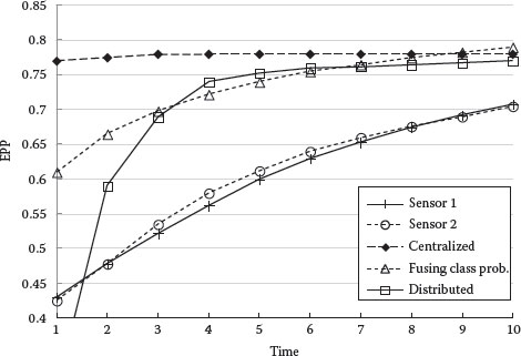
FIGURE 9.9 EPP of correct classification versus time.

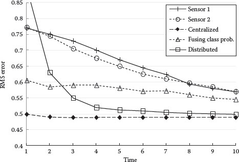
FIGURE 9.10 RMS object classification probability error versus time.

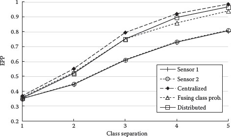
FIGURE 9.11 EPP of correct classification versus object class separation.

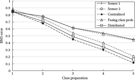
FIGURE 9.12 RMS object classification probability error versus object class separation.

Figures 9.13 and 9.14 show how the transition probability of the dynamic feature affects classification performance. Note that single sensor performance benefits more from increasing the transition probability than those of two sensors. This is probably due to better observability of the static feature from varying the dynamic feature. Larger transition probability implies more movement in viewing angles and better average observability.

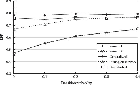
FIGURE 9.13 EPP of correct classification versus transition probability.

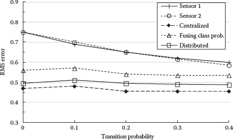
FIGURE 9.14 RMS classification probability error versus transition probability.

Figures 9.15 and 9.16 compare the performance of distributed classification using the adaptive and fixed schedule communication strategies. The results of centralized fusion, fusing object class probabilities, and single sensor classification are plotted for reference.

The adaptive communication strategy performs much better than the fixed schedule strategy, and achieves the performance of centralized fusion when the average number of communications is about 5. Fixed schedule communication does not achieve this level of performance with twice that number.

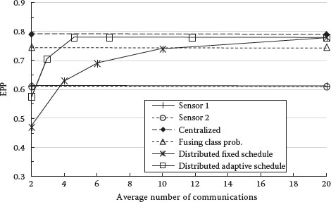
FIGURE 9.15 EPP of correct classification versus number of communications.

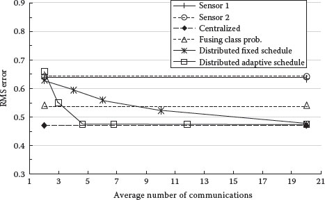
FIGURE 9.16 RMS classification probability error versus average number of communications.

9.7 CONCLUSIONS

Distributed object classification is an important problem in distributed data fusion and has been extensively studied by the fusion community. Technical issues are similar to those in distributed tracking and include choice of appropriate architecture, addressing dependent information in the data to be fused, design of optimal algorithms, etc. For the important cases involving imaging techniques, there are a number of additional issues not covered in this chapter that should be considered if imaging sensors are employed; there is an extensive body of literature on these problems. Here, we have discussed a range of foundational, architectural, and algorithmic issues that in fact can also be employed with imaging sensors but have not been explicitly framed in a sensor-specific way. We also present an approach for the important case of optimal distributed Bayesian classification and compare its performance with simpler fusion rules.

REFERENCES

Al-Ani, A. and M. Deriche. 2002. A new technique for combining multiple classifiers using the Dempster–Shafer theory of evidence. Journal of Artificial Intelligence Research, 17:333–361.

Bhanu, B. 1986. Automatic target recognition: State of the art survey. IEEE Transactions on Aerospace and Electronic Systems, 22:364–379.

Brooks, R. R., P. Ramanthan, and A. M. Sayed. 2003. Distributed target classification and tracking in sensor networks. Proceedings of IEEE, 91:1163–1171.

Chong, C. Y., K. C. Chang, and S. Mori. 2012. Fundamentals of distributed estimation. In Distributed Fusion for Net-Centric Operations, D. Hall, M. Liggins, C. Y. Chong, and J. Llinas (eds.). Boca Raton, FL: CRC Press.

Chong, C. Y. and S. Mori. 2004. Graphical models for nonlinear distributed estimation. Proceedings of the 7th International Conference on Information Fusion (FUSION 2004), Stockholm, Sweden, pp. 614–621.

Chong, C. Y. and S. Mori. 2005. Distributed fusion and communication management for target identification. Proceedings of the 8th International Conference on Information Fusion, Philadelphia, PA.

Chong, C. Y., S. Mori, and K. C. Chang. 1990. Distributed multitarget multisensor tracking. In Multitarget-Multisensor Tracking: Advanced Applications, Y. Bar-Shalom (ed.), chapter 8, pp. 247–295. Norwood, MA: Artech House.

Cohen, M. N. 1991. An overview of radar-based, automatic, noncooperative target recognition techniques. Proceedings of IEEE International Conference on Systems Engineering, Dayton, OH, pp. 29–34.

Duda, R. O., P. E. Hart, and D. G. Stork. 2001. Pattern Classification. New York: Wiley Interscience.

Hartshorne, C., P. Weiss, and A. Burks, eds. 1931–1958. The Collected Papers of Charles Sanders Peirce. Cambridge, MA: Harvard University Press.

Ho, T. K., J. H. Hull, and S. N. Srihari. 1994. Decision combination in multiple classifier systems. IEEE Transactions on Pattern Recognition and Machine Intelligence, 16:66–75.

Jensen, F. Y. 2001. Bayesian Networks and Decision Graphs. New York: Springer-Verlag.

Kittler, J., M. Hatef, R. P. W. Duin, and J. Matas. 1998. On combining classifiers. IEEE Transactions on Pattern Analysis and Machine Intelligence, 20:226–239.

Kotecha, J. H., V. Ramachandran, and A. M. Sayeed. 2005. Distributed multitarget classification in wireless sensor networks. IEEE Journal in Selected Areas in Communications, 23:703–713.

Kullback, S. and R. A. Leibler. 1951. On information and sufficiency. Annals of Mathematical Statistics, 22:79–86.

Kuncheva, L. I. 2002. A theoretical study on six classifier fusion strategies. IEEE Transactions on Pattern Analysis and Machine Intelligence, 24:281–286.

Liggins II, M., C. Y. Chong, I. Kadar, M. G. Alford, V. Vannicola, and S. Thomopoulos. 1997. Distributed fusion architectures and algorithms for target tracking. Proceedings IEEE, 85:95–107.

Llinas, J., R. Acharya, and C. Ke. 1998. Fusion-based methods in the absence of quantitative classifier confidence. Report CMIF 6–98, Center for Multisource Information Fusion, University at Buffalo, Buffalo, New York.

Montillo, A. 2010. Generative versus discriminative modeling frameworks. Lecture at Temple University http://www.albertmontillo.com/lectures,presentations/Generative%20vs%20Discriminative.pdf

Murphy, R. and B. Taylor. 2002. A survey of machine learning techniques for automatic target recognition, submitted to IEEE Transactions on Pattern Analysis and Machine Intelligence, www.citeseer.ist.psu.edu/viewdoc/summarydoi=10.1.1.53.9244

Nebabin, V. G. 1994. Methods and Techniques of Radar Recognition. Norwood, MA: Artech House.

Ng, A. Y. and M. I. Jordan. 2002. On discriminative vs. generative classifiers: A comparison of logistic regression and naive Bayes. Advances in Neural Information Processing Systems, 2:841–848.

Novak, L. M. 2000. State of the art of SAR automatic target recognition. Proceedings of the IEEE 2000 International Radar Conference, Alexandria, VA, pp. 836–843.

Pearl, J. 1988. Probabilistic Reasoning in Intelligent Systems: Networks of Plausible Inference. San Francisco, CA: Morgan Kaufman.

Roth, M. W. 1990. Survey of neural network technology for automatic target recognition. IEEE Transactions on Neural Networks, 1:28–43.

Ruta, D. and B. Gabrys. 2000. An overview of classifier fusion methods. Computing and Information Systems, 7:1–10.

Sadjadi, F. A. and B. Javidi. 2007. Physics of Automatic Target Recognition. New York: Springer.

Tait, P. 2005. Introduction to Radar Target Recognition (Radar, Sonar & Navigation). London, U.K.: The Institution of Engineering and Technology.

Zalta, E. N. ed. 2012. Stanford Encyclopedia of Philosophy. http://plato.stanford.edu/

* The term “labels” is generally used in the pattern recognition community to mean an object-class or class-type declaration; it could be considered a “vote” by a classifier in the context of an object-class label. If that vote or label is declared without an accompanying level of uncertainty, then such declaration is also called a “hard” declaration.

..................Content has been hidden....................

You can't read the all page of ebook, please click here login for view all page.

Table of Contents for Chapter 9 Object Classification in a Distributed Environment

Create new playlist

Sign In

Sign Up

Table of Contents for
Chapter 9 Object Classification in a Distributed Environment