
6
Advanced Optimization
You already know optimization. In Chapter 3, we covered gradient ascent/descent, which lets us “climb hills” to find a maximum or minimum. Any optimization problem can be thought of as a version of hill climbing: we strive to find the best possible outcome out of a huge range of possibilities. The gradient ascent tool is simple and elegant, but it has an Achilles’ heel: it can lead us to find a peak that is only locally optimal, not globally optimal. In the hill-climbing analogy, it might take us to the top of a foothill, when going downhill for just a little while would enable us to start scaling the huge mountain that we actually want to climb. Dealing with this issue is the most difficult and crucial aspect of advanced optimization.
In this chapter, we discuss a more advanced optimization algorithm using a case study. We’ll consider the traveling salesman problem, as well as several of its possible solutions and their shortcomings. Finally, we’ll introduce simulated annealing, an advanced optimization algorithm that overcomes these shortcomings and can perform global, rather than just local, optimization.
Life of a Salesman
The traveling salesman problem (TSP) is an extremely famous problem in computer science and combinatorics. Imagine that a traveling salesman wishes to visit a collection of many cities to peddle his wares. For any number of reasons—lost income opportunities, the cost of gas for his car, his head aching after a long journey (Figure 6-1)—it’s costly to travel between cities.

Figure 6-1: A traveling salesman in Naples
The TSP asks us to determine the order of travel between cities that will minimize travel costs. Like all the best problems in science, it’s easy to state and extremely difficult to solve.
Setting Up the Problem
Let’s fire up Python and start exploring. First, we’ll randomly generate a map for our salesman to traverse. We start by selecting some number N that will represent the number of cities we want on the map. Let’s say N = 40. Then we’ll select 40 sets of coordinates: one x value and one y value for each city. We’ll use the numpy module to do the random selection:
import numpy as np
random_seed = 1729
np.random.seed(random_seed)
N = 40
x = np.random.rand(N)
y = np.random.rand(N)
In this snippet, we used the numpy module’s random.seed() method. This method takes any number you pass to it and uses that number as a “seed” for its pseudorandom number generation algorithm (see Chapter 5 for more about pseudorandom number generation). This means that if you use the same seed we used in the preceding snippet, you’ll generate the same random numbers we generate here, so it will be easier to follow the code and you’ll get plots and results that are identical to these.
Next, we’ll zip the x values and y values together to create cities, a list containing the coordinate pair for each of our 40 randomly generated city locations.
points = zip(x,y)
cities = list(points)
If you run print(cities) in the Python console, you can see a list containing the randomly generated points. Each of these points represents a city. We won’t bother to give any city a name. Instead, we can refer to the first city as cities[0], the second as cities[1], and so on.
We already have everything we need to propose a solution to the TSP. Our first proposed solution will be to simply visit all the cities in the order in which they appear in the cities list. We can define an itinerary variable that will store this order in a list:
itinerary = list(range(0,N))This is just another way of writing the following:
itinerary = [0,1,2,3,4,5,6,7,8,9,10,11,12,13,14,15,16,17,18,19,20,21,22,23,24,25,26,27,28,29, 30,31,32,33,34,35,36,37,38,39]The order of the numbers in our itinerary is the order in which we’re proposing to visit our cities: first city 0, then city 1, and so on.
Next, we’ll need to judge this itinerary and decide whether it represents a good or at least acceptable solution to the TSP. Remember that the point of the TSP is to minimize the cost the salesman faces as he travels between cities. So what is the cost of travel? We can specify whatever cost function we want: maybe certain roads have more traffic than others, maybe there are rivers that are hard to cross, or maybe it’s harder to travel north than east or vice versa. But let’s start simply: let’s say it costs one dollar to travel a distance of 1, no matter which direction and no matter which cities we’re traveling between. We won’t specify any distance units in this chapter because our algorithms work the same whether we’re traveling miles or kilometers or light-years. In this case, minimizing the cost is the same as minimizing the distance traveled.
To determine the distance required by a particular itinerary, we need to define two new functions. First, we need a function that will generate a collection of lines that connect all of our points. After that, we need to sum up the distances represented by those lines. We can start by defining an empty list that we’ll use to store information about our lines:
lines = []Next, we can iterate over every city in our itinerary, at each step adding a new line to our lines collection that connects the current city and the city after it.
for j in range(0,len(itinerary) - 1):
    lines.append([cities[itinerary[j]],cities[itinerary[j + 1]]])
If you run print(lines), you can see how we’re storing information about lines in Python. Each line is stored as a list that contains the coordinates of two cities. For example, you can see the first line by running print(lines[0]), which will show you the following output:
[(0.21215859519373315, 0.1421890509660515), (0.25901824052776146, 0.4415438502354807)]We can put these elements together in one function called genlines (short for “generate lines”), which takes cities and itinerary as arguments and returns a collection of lines connecting each city in our list of cities, in the order specified in the itinerary:
def genlines(cities,itinerary):
    lines = []
    for j in range(0,len(itinerary) - 1):
        lines.append([cities[itinerary[j]],cities[itinerary[j + 1]]])
    return(lines)
Now that we have a way to generate a collection of lines between each two cities in any itinerary, we can create a function that measures the total distances along those lines. It will start by defining our total distance as 0, and then for every element in our lines list, it will add the length of that line to the distance variable. We’ll use the Pythagorean theorem to get these line lengths.
import math
def howfar(lines):
    distance = 0
    for j in range(0,len(lines)):
        distance += math.sqrt(abs(lines[j][1][0] - lines[j][0][0])**2 +
        abs(lines[j][1][1] - lines[j][0][1])**2)
    return(distance)
This function takes a list of lines as its input and outputs the sum of the lengths of every line. Now that we have these functions, we can call them together with our itinerary to determine the total distance our salesman has to travel:
totaldistance = howfar(genlines(cities,itinerary))
print(totaldistance)
When I ran this code, I found that the totaldistance was about 16.81. You should get the same results if you use the same random seed. If you use a different seed or set of cities, your results will vary slightly.
To get a sense of what this result means, it will help to plot our itinerary. For that, we can create a plotitinerary() function:
import matplotlib.collections as mc
import matplotlib.pylab as pl
def plotitinerary(cities,itin,plottitle,thename):
    lc = mc.LineCollection(genlines(cities,itin), linewidths=2)
    fig, ax = pl.subplots()
    ax.add_collection(lc)
    ax.autoscale()
    ax.margins(0.1)
    pl.scatter(x, y)
    pl.title(plottitle)
    pl.xlabel('X Coordinate')
    pl.ylabel('Y Coordinate')
    pl.savefig(str(thename) + '.png')
    pl.close()
The plotitinerary() function takes cities, itin, plottitle, and thename as arguments, where cities is our list of cities, itin is the itinerary we want to plot, plottitle is the title that will appear at the top of our plot, and thename is the name that we will give to the png plot output. The function uses the pylab module for plotting and matplotlib’s collections module to create a collection of lines. Then it plots the points of the itinerary and the lines we’ve created connecting them.
If you plot the itinerary with plotitinerary(cities,itinerary,'TSP - Random Itinerary','figure2'), you’ll generate the plot shown in Figure 6-2.

Figure 6-2: The itinerary resulting from visiting the cities in the random order in which they were generated
Maybe you can tell just by looking at Figure 6-2 that we haven’t yet found the best solution to the TSP. The itinerary we’ve given our poor salesman has him whizzing all the way across the map to an extremely distant city several times, when it seems obvious that he could do much better by stopping at some other cities along the way. The goal of the rest of this chapter is to use algorithms to find an itinerary with the minimum traveling distance.
The first potential solution we’ll discuss is the simplest and has the worst performance. After that, we’ll discuss solutions that trade a little complexity for a lot of performance improvement.
Brains vs. Brawn
It might occur to you to make a list of every possible itinerary that can connect our cities and evaluate them one by one to see which is best. If we want to visit three cities, the following is an exhaustive list of every order in which they can be visited:
- 1, 2, 3
- 1, 3, 2
- 2, 3, 1
- 2, 1, 3
- 3, 1, 2
- 3, 2, 1
It shouldn’t take long to evaluate which is best by measuring each of the lengths one by one and comparing what we find for each of them. This is called a brute force solution. It refers not to physical force, but to the effort of checking an exhaustive list by using the brawn of our CPUs rather than the brains of an algorithm designer, who could find a more elegant approach with a quicker runtime.
Sometimes a brute force solution is exactly the right approach. They tend to be easy to write code for, and they work reliably. Their major weakness is their runtime, which is never better and usually much worse than algorithmic solutions.
In the case of the TSP, the required runtime grows far too fast for a brute force solution to be practical for any number of cities higher than about 20. To see this, consider the following argument about how many possible itineraries there are to check if we are working with four cities and trying to find every possible order of visiting them:
- When we choose the first city to visit, we have four choices, since there are four cities and we haven’t visited any of them yet. So the total number of ways to choose the first city is 4.
- When we choose the second city to visit, we have three choices, since there are four cities total and we’ve already visited one of them. So the total number of ways to choose the first two cities is 4 × 3 = 12.
- When we choose the third city to visit, we have two choices, since there are four cities total and we’ve already visited two of them. So the total number of ways to choose the first three cities is 4 × 3 × 2 = 24.
- When we choose the fourth city to visit, we have one choice, since there are four cities total and we’ve already visited three of them. So the total number of ways to choose all four cities is 4 × 3 × 2 × 1 = 24.
You should’ve noticed the pattern here: when we have N cities to visit, the total number of possible itineraries is N × (N–1) × (N–2) × . . . × 3 × 2 × 1, otherwise known as N! (“N factorial”). The factorial function grows incredibly fast: while 3! is only 6 (which we can brute force without even using a computer), we find that 10! is over 3 million (easy enough to brute force on a modern computer), and 18! is over 6 quadrillion, 25! is over 15 septillion, and 35! and above starts to push the edge of what’s possible to brute force on today’s technology given the current expectation for the longevity of the universe.
This phenomenon is called combinatorial explosion. Combinatorial explosion doesn’t have a rigorous mathematical definition, but it refers to cases like this, in which apparently small sets can, when considered in combinations and permutations, lead to a number of possible choices far beyond the size of the original set and beyond any size that we know how to work with using brute force.
The number of possible itineraries that connect the 90 zip codes in Rhode Island, for example, is much larger than the estimated number of atoms in the universe, even though Rhode Island is much smaller than the universe. Similarly, a chess board can host more possible chess games than the number of atoms in the universe despite the fact that a chess board is even smaller than Rhode Island. These paradoxical situations, in which the nearly infinite can spring forth from the assuredly bounded, make good algorithm design all the more important, since brute force can never investigate all possible solutions of the hardest problems. Combinatorial explosion means that we have to consider algorithmic solutions to the TSP because we don’t have enough CPUs in the whole world to calculate a brute force solution.
The Nearest Neighbor Algorithm
Next we’ll consider a simple, intuitive method called the nearest neighbor algorithm. We start with the first city on the list. Then we simply find the closest unvisited city to the first city and visit that city second. At every step, we simply look at where we are and choose the closest unvisited city as the next city on our itinerary. This minimizes the travel distance at each step, although it may not minimize the total travel distance. Note that rather than looking at every possible itinerary, as we would in a brute force search, we find only the nearest neighbor at each step. This gives us a runtime that’s very fast even for very large N.
Implementing Nearest Neighbor Search
We’ll start by writing a function that can find the nearest neighbor of any given city. Suppose that we have a point called point and a list of cities called cities. The distance between point and the jth element of cities is given by the following Pythagorean-style formula:
point = [0.5,0.5]
j = 10
distance = math.sqrt((point[0] - cities[j][0])**2 + (point[1] - cities[j][1])**2)
If we want to find which element of cities is closest to our point (the point’s nearest neighbor), we need to iterate over every element of cities and check the distance between the point and every city, as in Listing 6-1.
def findnearest(cities,idx,nnitinerary):
    point = cities[idx]
    mindistance = float('inf')
    minidx = - 1
    for j in range(0,len(cities)):
        distance = math.sqrt((point[0] - cities[j][0])**2 + (point[1] - cities[j][1])**2)
        if distance < mindistance and distance > 0 and j not in nnitinerary:
            mindistance = distance
            minidx = j
    return(minidx)
Listing 6-1: The findnearest() function, which finds the nearest city to a given city
After we have this findnearest() function, we’re ready to implement the nearest neighbor algorithm. Our goal is to create an itinerary called nnitinerary. We’ll start by saying that the first city in cities is where our salesman starts:
nnitinerary = [0]If our itinerary needs to have N cities, our goal is to iterate over all the numbers between 0 and N – 1, find for each of those numbers the nearest neighbor to the most recent city we visited, and append that city to our itinerary. We’ll accomplish that with the function in Listing 6-2, donn() (short for “do nearest neighbor”). It starts with the first city in cities, and at every step adds the closest city to the most recently added city until every city has been added to the itinerary.
def donn(cities,N):
    nnitinerary = [0]
    for j in range(0,N - 1):
        next = findnearest(cities,nnitinerary[len(nnitinerary) - 1],nnitinerary)
        nnitinerary.append(next)
    return(nnitinerary)
Listing 6-2: A function that successively finds the nearest neighbor to each city and returns a complete itinerary
We already have everything we need to check the performance of the nearest neighbor algorithm. First, we can plot the nearest neighbor itinerary:
plotitinerary(cities,donn(cities,N),'TSP - Nearest Neighbor','figure3')Figure 6-3 shows the result we get.
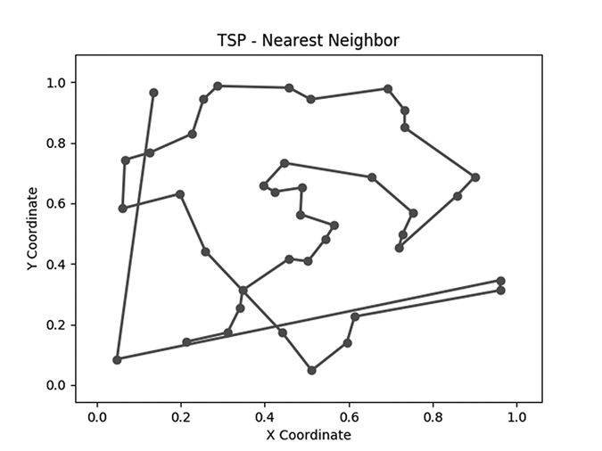
Figure 6-3: The itinerary generated by the nearest neighbor algorithm
We can also check how far the salesman had to travel using this new itinerary:
print(howfar(genlines(cities,donn(cities,N))))In this case, we find that whereas the salesman travels a distance of 16.81 following the random path, our algorithm has pushed down the distance to 6.29. Remember that we’re not using units, so we could interpret this as 6.29 miles (or kilometers or parsecs). The important thing is that it’s less than the 16.81 miles or kilometers or parsecs we found from the random itinerary. This is a significant improvement, all from a very simple, intuitive algorithm. In Figure 6-3, the performance improvement is evident; there are fewer journeys to opposite ends of the map and more short trips between cities that are close to each other.
Checking for Further Improvements
If you look closely at Figure 6-2 or Figure 6-3, you might be able to imagine some specific improvements that could be made. You could even attempt those improvements yourself and check whether they worked by using our howfar() function. For example, maybe you look at our initial random itinerary:
initial_itinerary = [0,1,2,3,4,5,6,7,8,9,10,11,12,13,14,15,16,17,18,19,20,21,22,23,24,25,26, 27,28,29,30,31,32,33,34,35,36,37,38,39]and you think you could improve the itinerary by switching the order of the salesman’s visits to city 6 and city 30. You can switch them by defining this new itinerary with the numbers in question switched (shown in bold):
new_itinerary = [0,1,2,3,4,5,30,7,8,9,10,11,12,13,14,15,16,17,18,19,20,21,22,23,24,25,26,27, 28,29,6,31,32,33,34,35,36,37,38,39]We can then do a simple comparison to check whether the switch we performed has decreased the total distance:
print(howfar(genlines(cities,initial_itinerary)))
print(howfar(genlines(cities,new_itinerary)))
If the new_itinerary is better than the initial_itinerary, we might want to throw out the initial_itinerary and keep the new one. In this case, we find that the new itinerary has a total distance of about 16.79, a very slight improvement on our initial itinerary. After finding one small improvement, we can run the same process again: pick two cities, exchange their locations in the itinerary, and check whether the distance has decreased. We can continue this process indefinitely, and at each step expect a reasonable chance that we can find a way to decrease the traveling distance. After repeating this process many times, we can (we hope) obtain an itinerary with a very low total distance.
It’s simple enough to write a function that can perform this switch-and-check process automatically (Listing 6-3):
def perturb(cities,itinerary):
    neighborids1 = math.floor(np.random.rand() * (len(itinerary)))
    neighborids2 = math.floor(np.random.rand() * (len(itinerary)))

    itinerary2 = itinerary.copy()

    itinerary2[neighborids1] = itinerary[neighborids2]
    itinerary2[neighborids2] = itinerary[neighborids1]

    distance1 = howfar(genlines(cities,itinerary))
    distance2 = howfar(genlines(cities,itinerary2))

    itinerarytoreturn = itinerary.copy()

    if(distance1 > distance2):
        itinerarytoreturn = itinerary2.copy()

    return(itinerarytoreturn.copy())
Listing 6-3: A function that makes a small change to an itinerary, compares it to the original itinerary, and returns whichever itinerary is shorter
The perturb() function takes any list of cities and any itinerary as its arguments. Then, it defines two variables: neighborids1 and neihborids2, which are randomly selected integers between 0 and the length of the itinerary. Next, it creates a new itinerary called itinerary2, which is the same as the original itinerary except that the cities at neighborids1 and neighborids2have switched places. Then it calculates distance1, the total distance of the original itinerary, and distance2, the total distance of itinerary2. If distance2 is smaller than distance1, it returns the new itinerary (with the switch). Otherwise, it returns the original itinerary. So we send an itinerary to this function, and it always returns an itinerary either as good as or better than the one we sent it. We call this function perturb() because it perturbs the given itinerary in an attempt to improve it.
Now that we have a perturb() function, let’s call it repeatedly on a random itinerary. In fact, let’s call it not just one time but 2 million times in an attempt to get the lowest traveling distance possible:
itinerary = [0,1,2,3,4,5,6,7,8,9,10,11,12,13,14,15,16,17,18,19,20,21,22,23,24,25,26,27,28,29, 30,31,32,33,34,35,36,37,38,39]

np.random.seed(random_seed)
itinerary_ps = itinerary.copy()
for n in range(0,len(itinerary) * 50000):
    itinerary_ps = perturb(cities,itinerary_ps)

print(howfar(genlines(cities,itinerary_ps)))
We have just implemented something that might be called a perturb search algorithm. It’s searching through many thousands of possible itineraries in the hopes of finding a good one, just like a brute force search. However, it’s better because while a brute force search would consider every possible itinerary indiscriminately, this is a guided search that is considering a set of itineraries that are monotonically decreasing in total traveling distance, so it should arrive at a good solution faster than brute force. We only need to make a few small additions to this perturb search algorithm in order to implement simulated annealing, the capstone algorithm of this chapter.
Before we jump into the code for simulated annealing, we’ll go over what kind of improvement it offers over the algorithms we’ve discussed so far. We also want to introduce a temperature function that allows us to implement the features of simulated annealing in Python.
Algorithms for the Avaricious
The nearest neighbor and perturb search algorithms that we’ve considered so far belong to a class of algorithms called greedy algorithms. Greedy algorithms proceed in steps, and they make choices that are locally optimal at each step but may not be globally optimal once all the steps are considered. In the case of our nearest neighbor algorithm, at each step, we look for the closest city to where we are at that step, without any regard to the rest of the cities. Visiting the closest city is locally optimal because it minimizes the distance we travel at the step we’re on. However, since it doesn’t take into account all cities at once, it may not be globally optimal—it may lead us to take strange paths around the map that eventually make the total trip extremely long and expensive for the salesman even though each individual step looked good at the time.
The “greediness” refers to the shortsightedness of this locally optimizing decision process. We can understand these greedy approaches to optimization problems with reference to the problem of trying to find the highest point in a complex, hilly terrain, where “high” points are analogous to better, optimal solutions (short distances in the TSP), and “low” points are analogous to worse, suboptimal solutions (long distances in the TSP). A greedy approach to finding the highest point in a hilly terrain would be to always go up, but that might take us to the top of a little foothill instead of the top of the highest mountain. Sometimes it’s better to go down to the bottom of the foothill in order to start the more important ascent of the bigger mountain. Because greedy algorithms search only for local improvements, they will never allow us to go down and can get us stuck on local extrema. This is exactly the problem discussed in Chapter 3.
With that understanding, we’re finally ready to introduce the idea that will enable us to resolve the local optimization problem caused by greedy algorithms. The idea is to give up the naive commitment to always climbing. In the case of the TSP, we may sometimes have to perturb to worse itineraries so that later we can get the best possible itineraries, just as we go down a foothill in order to ultimately go up a mountain. In other words, in order to do better eventually, we have to do worse initially.
Introducing the Temperature Function
To do worse with the intention of eventually doing better is a delicate undertaking. If we’re overzealous in our willingness to do worse, we might go downward at every step and get to a low point instead of a high one. We need to find a way to do worse only a little, only occasionally, and only in the context of learning how to eventually do better.
Imagine again that we’re in a complex, hilly terrain. We start in the late afternoon and know that we have two hours to find the highest point in the whole terrain. Suppose we don’t have a watch to keep track of our time, but we know that the air gradually cools down in the evening, so we decide to use the temperature as a way to gauge approximately how much time we have left to find the highest point.
At the beginning of our two hours, when it’s relatively hot outside, it is natural for us to be open to creative exploration. Since we have a long time remaining, it’s not a big risk to travel downward a little in order to understand the terrain better and see some new places. But as it gets cooler and we near the end of our two hours, we’ll be less open to broad exploration. We’ll be more narrowly focused on improvements and less willing to travel downward.
Take a moment to think about this strategy and why it’s the best way to get to the highest point. We already talked about why we want to go down occasionally: so that we can avoid a “local optimum,” or the top of a foothill next to a huge mountain. But when should we go down? Consider the last 10 seconds of our two-hour time period. No matter where we are, we should go as directly upward as we can at that time. It’s no use to go down to explore new foothills and find new mountains during our last 10 seconds, since even if we found a promising mountain, we wouldn’t have time to climb it, and if we make a mistake and slip downward during our last 10 seconds, we won’t have time to correct it. Thus, the last 10 seconds is when we should go directly up and not consider going down at all.
By contrast, consider the first 10 seconds of our two-hour time period. During that time, there’s no need to rush directly upward. At the beginning, we can learn the most from going a little downward to explore. If we make a mistake in the first 10 seconds, there’s plenty of time to correct it later. We’ll have plenty of time to take advantage of anything we learn or any mountains we find. During the first 10 seconds, it pays to be the most open about going down and the least zealous about going directly up.
You can understand the remainder of the two hours by thinking of the same ideas. If we consider the time 10 minutes before the end, we’ll have a more moderate version of the mindset we had 10 seconds before the end. Since the end is near, we’ll be motivated to go directly upward. However, 10 minutes is longer than 10 seconds, so we have some small amount of openness to a little bit of downward exploration just in case we discover something promising. By the same token, the time 10 minutes after the beginning will lead us to a more moderate version of the mindset we had 10 seconds after the beginning. The full two-hour time period will have a gradient of intention: a willingness to sometimes go down at first, followed by a gradually strengthening zeal to go only up.
In order to model this scenario in Python, we can define a function. We’ll start with a hot temperature and a willingness to explore and go downward, and we’ll end with a cool temperature and an unwillingness to go downward. Our temperature function is relatively simple. It takes t as an argument, where t stands for time:
temperature = lambda t: 1/(t + 1)You can see a simple plot of the temperature function by running the following code in the Python console. This code starts by importing matplotlib functionality and then defines ts, a variable containing a range of t values between 1 and 100. Finally, it plots the temperature associated with each t value. Again, we’re not worried about units or exact magnitude here because this is a hypothetical situation meant to show the general shape of a cooling function. So we use 1 to represent our maximum temperature, 0 to represent our minimum temperature, 0 to represent our minimum time, and 99 to represent our maximum time, without specifying units.
import matplotlib.pyplot as plt
ts = list(range(0,100))
plt.plot(ts, [temperature(t) for t in ts])
plt.title('The Temperature Function')
plt.xlabel('Time')
plt.ylabel('Temperature')
plt.show()
The plot looks like Figure 6-4.
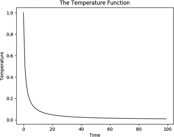
Figure 6-4: The temperature decreases as time goes on
This plot shows the temperature we’ll experience during our hypothetical optimization. The temperature is used as a schedule that will govern our optimization: our willingness to go down is proportional to the temperature at any given time.
We now have all the ingredients we need to fully implement simulated annealing. Go ahead—dive right in before you overthink it.
Simulated Annealing
Let’s bring all of our ideas together: the temperature function, the search problem in hilly terrain, the perturb search algorithm, and the TSP. In the context of the TSP, the complex, hilly terrain that we’re in consists of every possible solution to the TSP. We can imagine that a better solution corresponds to a higher point in the terrain, and a worse solution corresponds to a lower point in the terrain. When we apply the perturb() function, we’re moving to a different point in the terrain, hoping that point is as high as possible.
We’ll use the temperature function to guide our exploration of this terrain. When we start, our high temperature will dictate more openness to choosing a worse itinerary. Closer to the end of the process, we’ll be less open to choosing worse itineraries and more focused on “greedy” optimization.
The algorithm we’ll implement, simulated annealing, is a modified form of the perturb search algorithm. The essential difference is that in simulated annealing, we’re sometimes willing to accept itinerary changes that increase the distance traveled, because this enables us to avoid the problem of local optimization. Our willingness to accept worse itineraries depends on the current temperature.
Let’s modify our perturb() function with this latest change. We’ll add a new argument: time, which we’ll have to pass to perturb(). The time argument measures how far we are through the simulated annealing process; we start with time 1 the first time we call perturb(), and then time will be 2, 3, and so on as many times as we call the perturb() function. We’ll add a line that specifies the temperature function and a line that selects a random number. If the random number is lower than the temperature, then we’ll be willing to accept a worse itinerary. If the random number is higher than the temperature, then we won’t be willing to accept a worse itinerary. That way, we’ll have occasional, but not constant, times when we accept worse itineraries, and our likelihood of accepting a worse itinerary will decrease over time as our temperature cools. We’ll call this new function perturb_sa1(), where sa is short for simulated annealing. Listing 6-4 shows our new perturb_sa1() function with these changes.
def perturb_sa1(cities,itinerary,time):
    neighborids1 = math.floor(np.random.rand() * (len(itinerary)))
    neighborids2 = math.floor(np.random.rand() * (len(itinerary)))

    itinerary2 = itinerary.copy()

    itinerary2[neighborids1] = itinerary[neighborids2]
    itinerary2[neighborids2] = itinerary[neighborids1]

    distance1 = howfar(genlines(cities,itinerary))
    distance2 = howfar(genlines(cities,itinerary2))

    itinerarytoreturn = itinerary.copy()

    randomdraw = np.random.rand()
    temperature = 1/((time/1000) + 1)

    if((distance2 > distance1 and (randomdraw) < (temperature)) or (distance1 > distance2)):
        itinerarytoreturn=itinerary2.copy()

    return(itinerarytoreturn.copy())
Listing 6-4: An updated version of our perturb() function that takes into account the temperature and a random draw
Just by adding those two short lines, a new argument, and a new if condition (all shown in bold in Listing 6-4), we already have a very simple simulated annealing function. We also changed the temperature function a little; because we’ll be calling this function with very high time values, we use time/1000 instead of time as part of the denominator argument in our temperature function. We can compare the performance of simulated annealing with the perturb search algorithm and the nearest neighbor algorithm as follows:
itinerary = [0,1,2,3,4,5,6,7,8,9,10,11,12,13,14,15,16,17,18,19,20,21,22,23,24,25,26,27,28,29, 30,31,32,33,34,35,36,37,38,39]
np.random.seed(random_seed)

itinerary_sa = itinerary.copy()
for n in range(0,len(itinerary) * 50000):
    itinerary_sa = perturb_sa1(cities,itinerary_sa,n)

print(howfar(genlines(cities,itinerary))) #random itinerary
print(howfar(genlines(cities,itinerary_ps))) #perturb search
print(howfar(genlines(cities,itinerary_sa))) #simulated annealing
print(howfar(genlines(cities,donn(cities,N)))) #nearest neighbor
Congratulations! You can perform simulated annealing. You can see that a random itinerary has distance 16.81, while a nearest neighbor itinerary has distance 6.29, just like we observed before. The perturb search itinerary has distance 7.38, and the simulated annealing itinerary has distance 5.92. In this case, we’ve found that perturb search performs better than a random itinerary, that nearest neighbor performs better than perturb search and a random itinerary, and simulated annealing performs better than all the others. When you try other random seeds, you may see different results, including cases where simulated annealing does not perform as well as nearest neighbor. This is because simulated annealing is a sensitive process, and several aspects of it need to be tuned precisely in order for it to work well and reliably. After we do that tuning, it will consistently give us significantly better performance than simpler, greedy optimization algorithms. The rest of the chapter is concerned with the finer details of simulated annealing, including how to tune it to get the best possible performance.
Tuning Our Algorithm
As mentioned, simulated annealing is a sensitive process. The code we’ve introduced shows how to do it in a basic way, but we’ll want to make changes to the details in order to do better. This process of changing small details or parameters of an algorithm in order to get better performance without changing its main approach is often called tuning, and it can make big differences in difficult cases like this one.
Our perturb() function makes a small change in the itinerary: it switches the place of two cities. But this isn’t the only possible way to perturb an itinerary. It’s hard to know in advance which perturbing methods will perform best, but we can always try a few.
Another natural way to perturb an itinerary is to reverse some portion of it: take a subset of cities, and visit them in the opposite order. In Python, we can implement this reversal in one line. If we choose two cities in the itinerary, with indices small and big, the following snippet shows how to reverse the order of all the cities between them:
small = 10
big = 20
itinerary = [0,1,2,3,4,5,6,7,8,9,10,11,12,13,14,15,16,17,18,19,20,21,22,23,24,25,26,27,28,29, 30,31,32,33,34,35,36,37,38,39]
itinerary[small:big] = itinerary[small:big][::-1]
print(itinerary)
When you run this snippet, you can see that the output shows an itinerary with cities 10 through 19 in reverse order:
[0, 1, 2, 3, 4, 5, 6, 7, 8, 9, 19, 18, 17, 16, 15, 14, 13, 12, 11, 10, 20, 21, 22, 23, 24, 25, 26, 27, 28, 29, 30, 31, 32, 33, 34, 35, 36, 37, 38, 39]Another way to perturb an itinerary is to lift a section from where it is and place it in another part of the itinerary. For example, we might take the following itinerary:
itinerary = [0,1,2,3,4,5,6,7,8,9]and move the whole section [1,2,3,4] to later in the itinerary by converting it to the following new itinerary:
itinerary = [0,5,6,7,8,1,2,3,4,9]We can do this type of lifting and moving with the following Python snippet, which will move a chosen section to a random location:
small = 1
big = 5
itinerary = [0,1,2,3,4,5,6,7,8,9]
tempitin = itinerary[small:big]
del(itinerary[small:big])
np.random.seed(random_seed + 1)
neighborids3 = math.floor(np.random.rand() * (len(itinerary)))
for j in range(0,len(tempitin)):
    itinerary.insert(neighborids3 + j,tempitin[j])
We can update our perturb() function so that it randomly alternates between these different perturbing methods. We’ll do this by making another random selection of a number between 0 and 1. If this new random number lies in a certain range (say, 0–0.45), we’ll perturb by reversing a subset of cities, but if it lies in another range (say, 0.45–0.55), we’ll perturb by switching the places of two cities. If it lies in a final range (say, 0.55–1), we’ll perturb by lifting and moving a subset of cities. In this way, our perturb() function can randomly alternate between each type of perturbing. We can put this random selection and these types of perturbing into our new function, now called perturb_sa2(), as shown in Listing 6-5.
def perturb_sa2(cities,itinerary,time):
    neighborids1 = math.floor(np.random.rand() * (len(itinerary)))
    neighborids2 = math.floor(np.random.rand() * (len(itinerary)))

    itinerary2 = itinerary.copy()

    randomdraw2 = np.random.rand()
    small = min(neighborids1,neighborids2)
    big = max(neighborids1,neighborids2)
    if(randomdraw2 >= 0.55):
        itinerary2[small:big] = itinerary2[small:big][:: - 1]
    elif(randomdraw2 < 0.45):
        tempitin = itinerary[small:big]
        del(itinerary2[small:big])
        neighborids3 = math.floor(np.random.rand() * (len(itinerary)))
        for j in range(0,len(tempitin)):
            itinerary2.insert(neighborids3 + j,tempitin[j])
    else:
        itinerary2[neighborids1] = itinerary[neighborids2]
        itinerary2[neighborids2] = itinerary[neighborids1]

    distance1 = howfar(genlines(cities,itinerary))
    distance2 = howfar(genlines(cities,itinerary2))

    itinerarytoreturn = itinerary.copy()

    randomdraw = np.random.rand()
    temperature = 1/((time/1000) + 1)

    if((distance2 > distance1 and (randomdraw) < (temperature)) or (distance1 > distance2)):
        itinerarytoreturn = itinerary2.copy()

    return(itinerarytoreturn.copy())
Listing 6-5: Now, we use several different methods to perturb our itinerary.
Our perturb() function is now more complex and more flexible; it can make several different types of changes to itineraries based on random draws. Flexibility is not necessarily a goal worth pursuing for its own sake, and complexity is definitely not. In order to judge whether the complexity and flexibility are worth adding in this case (and in every case), we should check whether they improve performance. This is the nature of tuning: as with tuning a musical instrument, you don’t know beforehand exactly how tight a string needs to be—you have to tighten or loosen a little, listen to how it sounds, and adjust. When you test the changes here (shown in bold in Listing 6-5), you’ll be able to see that they do improve performance compared to the code we were running before.
Avoiding Major Setbacks
The whole point of simulated annealing is that we need to do worse in order to do better. However, we want to avoid making changes that leave us too much worse off. The way we set up the perturb() function, it will accept a worse itinerary any time our random selection is less than the temperature. It does this using the following conditional (which is not meant to be run alone):
if((distance2 > distance1 and randomdraw < temperature) or (distance1 > distance2)):We may want to change that condition so that our willingness to accept a worse itinerary depends not only on the temperature but also on how much worse our hypothetical change makes the itinerary. If it makes it just a little worse, we’ll be more willing to accept it than if it makes it much worse. To account for this, we’ll incorporate into our conditional a measurement of how much worse our new itinerary is. The following conditional (which is also not meant to be run alone) is an effective way to accomplish this:
scale = 3.5
if((distance2 > distance1 and (randomdraw) < (math.exp(scale*(distance1-distance2)) * temperature)) or (distance1 > distance2)):
When we put this conditional in our code, we have the function in Listing 6-6, where we show only the very end of the perturb() function.
--snip--
# beginning of perturb function goes here

    scale = 3.5
    if((distance2 > distance1 and (randomdraw) < (math.exp(scale * (distance1 - distance2)) * temperature)) or (distance1 > distance2)):
        itinerarytoreturn = itinerary2.copy()

    return(itinerarytoreturn.copy())
Allowing Resets
During the simulated annealing process, we may unwittingly accept a change to our itinerary that’s unequivocally bad. In that case, it may be useful to keep track of the best itinerary we’ve encountered so far and allow our algorithm to reset to that best itinerary under certain conditions. Listing 6-6 provides the code to do this, highlighted in bold in a new, full perturbing function for simulated annealing.
def perturb_sa3(cities,itinerary,time,maxitin):
    neighborids1 = math.floor(np.random.rand() * (len(itinerary)))
    neighborids2 = math.floor(np.random.rand() * (len(itinerary)))
    global mindistance
    global minitinerary
    global minidx
    itinerary2 = itinerary.copy()
    randomdraw = np.random.rand()

    randomdraw2 = np.random.rand()
    small = min(neighborids1,neighborids2)
    big = max(neighborids1,neighborids2)
    if(randomdraw2>=0.55):
        itinerary2[small:big] = itinerary2[small:big][::- 1 ]
    elif(randomdraw2 < 0.45):
        tempitin = itinerary[small:big]
        del(itinerary2[small:big])
        neighborids3 = math.floor(np.random.rand() * (len(itinerary)))
        for j in range(0,len(tempitin)):
            itinerary2.insert(neighborids3 + j,tempitin[j])
    else:
        itinerary2[neighborids1] = itinerary[neighborids2]
        itinerary2[neighborids2] = itinerary[neighborids1]

    temperature=1/(time/(maxitin/10)+1)

    distance1 = howfar(genlines(cities,itinerary))
    distance2 = howfar(genlines(cities,itinerary2))

    itinerarytoreturn = itinerary.copy()

    scale = 3.5
    if((distance2 > distance1 and (randomdraw) < (math.exp(scale*(distance1 - distance2)) * 	emperature)) or (distance1 > distance2)):
        itinerarytoreturn = itinerary2.copy()

    reset = True
    resetthresh = 0.04
    if(reset and (time - minidx) > (maxitin * resetthresh)):
        itinerarytoreturn = minitinerary
        minidx = time

    if(howfar(genlines(cities,itinerarytoreturn)) < mindistance):
        mindistance = howfar(genlines(cities,itinerary2))
        minitinerary = itinerarytoreturn
        minidx = time

    if(abs(time - maxitin) <= 1):
        itinerarytoreturn = minitinerary.copy()

    return(itinerarytoreturn.copy())
Listing 6-6: This function performs the full simulated annealing process and returns an optimized itinerary.
Here, we define global variables for the minimum distance achieved so far, the itinerary that achieved it, and the time at which it was achieved. If the time progresses very far without finding anything better than the itinerary that achieved our minimum distance, we can conclude that the changes we made after that point were mistakes, and we allow resetting to that best itinerary. We’ll reset only if we’ve attempted many perturbations without finding an improvement on our previous best, and a variable called resetthresh will determine how long we should wait before resetting. Finally, we add a new argument called maxitin, which tells the function how many total times we intend to call this function, so that we know where exactly in the process we are. We use maxitin in our temperature function as well so that the temperature curve can adjust flexibly to however many perturbations we intend to perform. When our time is up, we return the itinerary that gave us the best results so far.
Testing Our Performance
Now that we have made these edits and improvements, we can create a function called siman() (short for simulated annealing), which will create our global variables, and then call our newest perturb() function repeatedly, eventually arriving at an itinerary with a very low traveling distance (Listing 6-7).
def siman(itinerary,cities):
    newitinerary = itinerary.copy()
    global mindistance
    global minitinerary
    global minidx
    mindistance = howfar(genlines(cities,itinerary))
    minitinerary = itinerary
    minidx = 0

    maxitin = len(itinerary) * 50000
    for t in range(0,maxitin):
        newitinerary = perturb_sa3(cities,newitinerary,t,maxitin)

    return(newitinerary.copy())
Listing 6-7: This function performs the full simulated annealing process and returns an optimized itinerary.
Next, we call our siman() function and compare its results to the results of our nearest neighbor algorithm:
np.random.seed(random_seed)
itinerary = list(range(N))
nnitin = donn(cities,N)
nnresult = howfar(genlines(cities,nnitin))
simanitinerary = siman(itinerary,cities)
simanresult = howfar(genlines(cities,simanitinerary))
print(nnresult)
print(simanresult)
print(simanresult/nnresult)
When we run this code, we find that our final simulated annealing function yields an itinerary with distance 5.32. Compared to the nearest-neighbor itinerary distance of 6.29, this is an improvement of more than 15 percent. This may seem underwhelming to you: we spent more than a dozen pages grappling with difficult concepts only to shave about 15 percent from our total distance. This is a reasonable complaint, and it may be that you never need to have better performance than the performance offered by the nearest neighbor algorithm. But imagine offering the CEO of a global logistics company like UPS or DHL a way to decrease travel costs by 15 percent, and seeing the pupils of their eyes turn to dollar signs as they think of the billions of dollars this would represent. Logistics remains a major driver of high costs and environmental pollution in every business in the world, and doing well at solving the TSP will always make a big practical difference. Besides this, the TSP is extremely important academically, as a benchmark for comparing optimization methods and as a gateway to investigating advanced theoretical ideas.
You can plot the itinerary we got as the final result of simulated annealing by running plotitinerary(cities,simanitinerary,'Traveling Salesman Itinerary - Simulated Annealing','figure5'). You’ll see the plot in Figure 6-5.
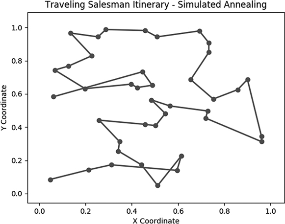
Figure 6-5: The final result of simulated annealing
On one hand, it’s just a plot of randomly generated points with lines connecting them. On the other, it’s the result of an optimization process that we performed over hundreds of thousands of iterations, relentlessly pursuing perfection among nearly infinite possibilities, and in that way it is beautiful.
Summary
In this chapter, we discussed the traveling salesman problem as a case study in advanced optimization. We discussed a few approaches to the problem, including brute force search, nearest neighbor search, and finally simulated annealing, a powerful solution that enables doing worse in order to do better. I hope that by working through the difficult case of the TSP, you have gained skills that you can apply to other optimization problems. There will always be a practical need for advanced optimization in business and in science.
In the next chapter, we turn our attention to geometry, examining powerful algorithms that enable geometric manipulations and constructions. Let the adventure continue!