The gdb package is available from ftp://ftp.gnu.org/gnu/gdb/ under the terms of the GPL. Download and extract the gdb package in your ${PRJROOT}/debug directory. For my control module, for example, I used gdb Version 5.2.1. As with the other GNU toolset components I described in Chapter 4, it is preferable not to use the package’s directory to build the actual debugger. Instead, create a build directory, move to it, and build gdb:

$ mkdir ${PRJROOT}/debug/build-gdb
$ cd ${PRJROOT}/debug/build-gdb
$ ../gdb-5.2.1/configure --target=$TARGET --prefix=${PREFIX}
$ make
$ make install

These commands build the gdb debugger for handling target applications. As with other GNU toolset components, the name of the binary depends on the target. For my control module, for example, the debugger is powerpc-linux-gdb. This binary and the other debugger files are installed within the $PREFIX directory. The build process proper takes from 5 to 10 minutes on my hardware, and the binary generated is fairly large. For a PPC target, for example, the stripped binary is 4 MB in size when linked dynamically. This is why the gdb binary can’t be used as-is on the target and the gdb server is used instead.

The gdb server wasn’t built earlier because it has to be cross-compiled for the target using the appropriate tools. To do so, create a directory to build the gdb server, move to it, and build the gdb server:

$ mkdir ${PRJROOT}/debug/build-gdbserver
$ cd ${PRJROOT}/debug/build-gdbserver
$ chmod +x ../gdb-5.2.1/gdb/gdbserver/configure
$ CC=powerpc-linux-gcc ../gdb-5.2.1/gdb/gdbserver/configure 
               > --host=$TARGET --prefix=${TARGET_PREFIX}
$ make
$ make install

The gdb server binary, gdbserver, has now been installed in your ${TARGET_PREFIX}/bin directory. The dynamically linked gdbserver is 25 KB in size when stripped. Compared to gdb, the size of gdbserver is much more palatable.

Once built, copy gdbserver to your target’s root filesystem:

$ cp ${TARGET_PREFIX}/bin/gdbserver ${PRJROOT}/rootfs/usr/bin

There are no additional steps required to configure the use of the gdb server on your target. I will cover its use in the next section.

$ powerpc-linux-readelf -S gdbserver
There are 32 section headers, starting at offset 0x1aca4:
Section Headers:
  [Nr] Name            Type           Addr     Off    Size   ES Flg Lk Inf Al
...
  [12] .text           PROGBITS       10000b48 000b48 003008 00  AX   0   0 4
...
  [17] .data           PROGBITS       10015470 005470 000914 00  WA   0   0 4
...
  [25] .bss            NOBITS         10016114 005e54 00236c 00  WA   0   0 16
  [26] .stab           PROGBITS       00000000 005e54 00798c 0c      27   0 4
  [27] .stabstr        STRTAB         00000000 00d7e0 00d1d5 00       0   0 1
  [28] .comment        PROGBITS       00000000 01a9b5 0001ee 00       0   0 1
  [29] .shstrtab       STRTAB         00000000 01aba3 0000ff 00       0   0 1
  [30] .symtab         SYMTAB         00000000 01b1a4 000f40 10      31  6e 4
  [31] .strtab         STRTAB         00000000 01c0e4 000d19 00       0   0 1
Key to Flags: W (write), A (alloc), X (execute), M (merge), S (strings)
              I (info), L (link order), O (extra OS processing required)
              o (os specific), p (processor specific) x (unknown)

$ powerpc-linux-readelf -S gdbserver
There are 28 section headers, starting at offset 0x6134:
Section Headers:
  [Nr] Name            Type           Addr     Off    Size   ES Flg Lk Inf Al
...
  [12] .text           PROGBITS       10000b48 000b48 003008 00  AX   0   0 4
...
  [17] .data           PROGBITS       10015470 005470 000914 00  WA   0   0 4
...
  [25] .bss            NOBITS         10016114 005e54 00236c 00  WA   0   0 16
  [26] .comment        PROGBITS       00000000 005e54 0001ee 00       0   0 1
  [27] .shstrtab       STRTAB         00000000 006042 0000f0 00       0   0 1
Key to Flags: W (write), A (alloc), X (execute), M (merge), S (strings)
              I (info), L (link order), O (extra OS processing required)
              o (os specific), p (processor specific) x (unknown)

Before you can debug an application using gdb, you need to compile your application using the appropriate flags. Mainly, you need to add the -g option to the gcc command line. This option adds the debugging information to the object files generated by the compiler. To add even more debugging information, use the -ggdb option. The information added by both debugging options is thereafter found in the application’s binary. Though this addition results in a larger binary, you can still use a stripped binary on your target, granted you have the original unstripped version with the debugging information on your host. To do so, build your application on your host with complete debugging symbols. Copy the resulting binary to your target’s root filesystem and use strip to reduce the size of the binary you just copied by removing all symbolic information, including debugging information. On the target, use the stripped binary with gdbserver. On the host, use the original unstripped binary with gdb. Though the two gdb components are using different binary images, the target gdb running on the host is able to find and use the appropriate debug symbols for your application, because it has access to the unstripped binary.

Here are the relevant portions of my command daemon’s Makefile that changed (see Chapter 4 for the original Makefile):

               ...
DEBUG         = -g
CFLAGS        = -O2 -Wall $(DEBUG)
...

Though gcc allows us to use both the -g and -O options in the same time, it is often preferable not to use the -O option when generating a binary for debugging, because the optimized binary may contain some subtle differences when compared to your application’s original source code. For instance, some unused variables may not be incorporated into the binary, and the sequence of instructions actually executed in the binary may differ in order from those contained in your original source code.

There are two ways for the gdb server running on the target to communicate with the gdb debugger running on the host: using a crossover serial link or a TCP/IP connection. Though these communication interfaces differ in many respects, the syntax of the commands you need to issue is very similar. Starting a debug session using a gdb server involves two steps: starting the gdb server on the target and connecting to it from the gdb debugger on the host.

Once you are ready to debug your application, start the gdb server on your target with the means of communication and your application name as parameters. If your target has a configured TCP/IP interface available, you can start the gdb server and configure it to run over TCP/IP:

# gdbserver 192.168.172.50:2345 command-daemon

In this example, the host’s IP address^[2] is 192.168.172.50 and the port number used locally to listen to gdb connections is 2345. Note that the protocol used by gdb to communicate between the host and the target doesn’t include any form of authentication or security. Hence, I don’t recommend that you debug applications in this way over the public Internet. If you need to debug applications in this way, you may want to consider using SSH port forwarding to encrypt the gdb session. The book SSH, The Secure Shell: The Definitive Guide (O’Reilly) explains how to implement SSH port forwarding.

As I said earlier, the command-daemon being passed to gdbserver can be a stripped copy of the original command-daemon built on the host.

If you are using a serial link to debug your target, use the following command line on your target:

# gdbserver /dev/ttyS0 command-daemon

In this example, the target’s serial link to the host is the first serial port, /dev/ttyS0.

Once the gdb server is started on the target, you can connect to it from the gdb debugger on the host using the target remote command. If you are connected to the target using a TCP/IP network, use the following command:

$ powerpc-linux-gdb command-daemon
(gdb) target remote 192.168.172.10:2345
Remote debugging using 192.168.172.10:2345
0x10000074 in _start (  )

In this case, the target is located at IP 192.168.172.10 and the port number specified is the same one we used above to start the gdb server on the target. Unlike the gdb server on the target, the command-daemon used here has to be the unstripped copy of the binary. Otherwise, gdb will be of little use to try debugging the application.

If the program exits on the target or is restarted, you do not need to restart gdb on the host. Instead, you need to issue the target remote command anew once gdbserver is restarted on the target.

If your host is connected to your target through a serial link, use the following command:

$ powerpc-linux-gdb progname
(gdb) target remote /dev/ttyS0
Remote debugging using /dev/ttyS0
0x10000074 in _start (  )

Though both the target and the host are using /dev/ttyS0 to link to each other in this example, this is only a coincidence. The target and the host can use different serial ports to link to each other. The device being specified for each is the local serial port where the serial cable is connected.

With the target and the host connected, you can now set breakpoints and do anything you would normally do in a symbolic debugger.

There are a few gdb commands that are you are likely to find particularly useful when debugging an embedded target such as we are doing here. Here are some of these commands and summaries of their purposes:

The last command is likely to be the most useful when your binaries are linked dynamically. Whereas the binary running on your target finds its shared libraries starting from / (the root directory), the gdb running on the host doesn’t know how to locate these shared libraries. You need to use the following command to tell gdb where to find the correct target libraries on the host:

(gdb) set solib-absolute-prefix ../../tools/powerpc-linux/

Unlike the normal shell, the gdb command line doesn’t recognize environment variables such as ${TARGET_PREFIX}. Hence, the complete path must be provided. In this case, the path is provided relative to the directory where gdb is running, but we could use an absolute path, too.

If you want to have gdb execute a number of commands each time it starts, you may want to use a .gdbinit file. For an explanation on the use of such files, have a look at the “Command files” subsection in the “Canned Sequences of Commands” section of the gdb manual.

To get information regarding the use of the various debugger commands, you can use the help command within the gdb environment, or look in the gdb manual.

Many developers find it difficult or counter-intuitive to debug using the plain gdb command line. Fortunately for these developers, there are quite a few graphical interfaces that hide much of gdb’s complexity by providing user-friendly mechanisms for setting breakpoints, viewing variables, and tending to other common debugging tasks. Examples include DDD (http://www.gnu.org/software/ddd/), KDevelop and other IDEs we discussed in Chapter 4. Much like your host’s debugger, the cross-platform gdb we built earlier for your target can very likely be used by your favorite debugging interface. Each frontend has its own way for allowing the name of the debugger binary to be specified. Have a look at your frontend’s documentation for this information. In the case of my control module, I would need to configure the frontend to use the powerpc-linux-gdb debugger.

The main tool for tracing a single process is strace. strace uses the ptrace( ) system call to intercept all system calls made by an application. Hence, it can extract all the system call information and display it in a human-readable format for you to analyze. Because strace is a widely used Linux tool, I do not explain how to use it, but just explain how to install it for your target. If you would like to have more details on the usage of strace, see Chapter 14 of Running Linux.

strace is available from http://www.liacs.nl/~wichert/strace/ under a BSD license. For my control module I used strace Version 4.4. Download the package and extract it in your ${PRJROOT}/debug directory. Move to the package’s directory, then configure and build strace:

$ cd ${PRJROOT}/debug/strace-4.4
$ CC=powerpc-linux-gcc ./configure --host=$TARGET
$ make

If you wish to statically link against uClibc, add LDFLAGS="-static" to the make command line. Given that strace uses NSS, you need to use a special command line if you wish to link it statically to glibc, as we did for other packages in Chapter 10:

$ make 
               > LDLIBS="-static -Wl --start-group -lc -lnss_files -lnss_dns 
               > -lresolv -Wl --end-group"

When linked against glibc and stripped, strace is 145 KB in size if linked dynamically and 605 KB if linked statically. When linked against uClibc and stripped, strace is 140 KB in size if linked dynamically and 170 KB when linked statically.

Once the binary is compiled, copy it to your target’s root filesystem:

$ cp strace ${PRJROOT}/rootfs/usr/sbin

There are no additional steps required to configure strace for use on the target. In addition, the use of strace on the target is identical to that of its use on a normal Linux workstation. See the web page listed earlier or the manpage included with the package if you need more information regarding the use of strace.

The main system tracing utility for Linux is the Linux Trace Toolkit (LTT), which was introduced and continues to be maintained by this book’s author. In contrast with other tracing utilities such as strace, LTT does not use the ptrace( ) mechanism to intercept applications’ behavior. Instead, a kernel patch is provided with LTT that instruments key kernel subsystems. The data generated by this instrumentation is then collected by the trace subsystem and forwarded to a trace daemon to be written to disk. The entire process has very little impact on the system’s behavior and performance. Extensive tests have shown that the tracing infrastructure has marginal impact when not in use and an impact lower than 2.5% under some of the most stressful conditions.

In addition to reconstructing the system’s behavior using the data generated during a trace run, the user utilities provided with LTT allow you to extract performance data regarding the system’s behavior during the trace interval. Here’s a summary of some of the tasks LTT can be used for:

To achieve this, LTT’s operation is subdivided into four software components:

The first two software components are implemented as a kernel patch and the last two are separate user-space tools. While the first three software components must run on the target, the last one, the visualization tool, can run on the host. In LTT Versions 0.9.5a and earlier, the tracing subsystem was accessed from user space as a device through the appropriate /dev entries. Starting in the development series leading to 0.9.6, however, this abstraction has been dropped following the recommendations of the kernel developers. Hence, though the following refers to the tracing subsystem as a device, newer versions of LTT will not use this abstraction and therefore will not require the creation of any /dev entries on your target’s root filesystem.

Given that LTT can detect and handle traces that have different byte ordering, traces can be generated and read on entirely different systems. The traces generated on my PPC-based control module, for example, can be read transparently on an x86 host.

In addition to tracing a predefined set of events, LTT enables you to create and log your own custom events from both user space and kernel space. Have a look at the Examples directory included in the package for practical examples of such custom events. Also, if your target is an x86-or PPC-based system, you can use the DProbes package provided by IBM to add trace points to binaries, including the kernel, without recompiling. DProbes is available under the terms of the GPL from IBM’s web site at http://oss.software.ibm.com/developer/opensource/linux/projects/dprobes/.

LTT is available under the terms of the GPL from Opersys’s web site at http://www.opersys.com/LTT/. The project’s web site includes links to in-depth documentation and a mailing list for LTT users. The current stable release is 0.9.5a, which supports the i386, PPC, and SH architectures. The 0.9.6 release currently in development adds support for the MIPS and the ARM architectures.

$ cd ${PRJROOT}/debug
$ tar xvzf TraceToolkit-0.9.5a.tgz
$ cd ${PRJROOT}/debug/TraceToolkit-0.9.5

$ mv patch-ltt-linux-2.4.19-vanilla-020916-1.14 
                  > ${PRJROOT}/kernel/linux-2.4.18
$ cd ${PRJROOT}/kernel/linux-2.4.18
$ patch -p1 < patch-ltt-linux-2.4.19-vanilla-020916-1.14

$ cd ${PRJROOT}/debug/TraceToolkit-0.9.5
$ ./configure --prefix=${PREFIX}
$ make -C LibUserTrace CC=powerpc-linux-gcc UserTrace.o
$ make -C LibUserTrace CC=powerpc-linux-gcc LDFLAGS="-static"
$ make -C Daemon CC=powerpc-linux-gcc LDFLAGS="-static"

$ make -C Daemon CC=powerpc-linux-gcc LDFLAGS="-all-static"

$ cp tracedaemon Scripts/trace Scripts/tracecore Scripts/traceu 
                  > ${PRJROOT}/rootfs/usr/sbin

$ su -m
Password:
# mknod ${PRJROOT}/rootfs/dev/tracer c 254 0
# mknod ${PRJROOT}/rootfs/dev/tracerU c 254 1
# exit

$ make -C LibLTT install
$ make -C Visualizer install

Tracing the target and visualizing its behavior

You are now ready to trace your target. As I said earlier, to reduce wear, avoid using your target’s solid-state storage device for recording the traces. Instead, either write the traces to an NFS-mounted filesystem or, if you would prefer to reduce polluting the traces with NFS-generated network traffic, use a TMPFS mounted directory to store the traces and copy them to your host after tracing is over.

Here is a simple command for tracing the target for 30 seconds:

# trace 30 outt

The outt name specified here is the prefix the command should use for the names of the output files. This command will generate two files: outt.trace, which contains the raw binary trace, and outt.proc, which contains a snapshot of the system’s state at trace start. Both these files are necessary for reconstructing the system’s behavior on the host using the visualization tool. If those files are stored locally on your target, copy them to your host using your favorite protocol.

It is possible that your system may be generating more events than the trace infrastructure can handle. In that case, the daemon will inform you upon exit that it lost events. You can then change the size of the buffers being used or the event set being traced to obtain all the data you need. Look at the documentation included in the package for more information on the parameters accepted by the trace daemon.

Once you’ve copied the files containing the trace to the host, you can view the trace using:

$ traceview outt

This command opens a window that looks like Figure 11-1.

Figure 11-1. Example LTT trace graph

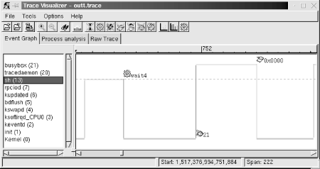
In this case, the graph shows the interaction between the BusyBox shell and another BusyBox child. On the left side of the visualizer display, you see a list of all the processes that were active during the trace. The Linux kernel is always the bottom entry in that list. On the right side of the display, you see a graph that characterizes the behavior of the system. In that graph, horizontal lines illustrate the passage of time, while vertical lines illustrate a state transition. The graph portion displayed here shows that the system is running kernel code in the beginning. Near the start, the kernel returns control to the sh application, which continues running for a short period of time before making the wait4( ) system call. At that point, control is transferred back to the kernel, which runs for a while before initiating a scheduling change to the task with PID 21. This task starts executing, but an exception occurs, which results in a control transfer to the kernel again.

The graph continues in both directions, and you can scroll left or right to see what happened before or after this trace segment. You can also zoom in and out, depending on your needs.

Using this sort of graph, you can easily identify your applications’ interaction with the rest of the system, as I explained earlier. You can also view the same set of events in their raw form by selecting the “Raw Trace” thumbnail, as seen in Figure 11-2.

Figure 11-2. Example LTT raw event list

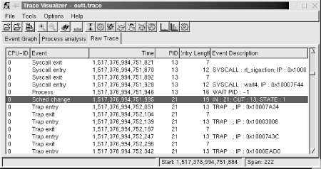
If you would prefer not to use the graphic tool at all, you can use the tracevisualizer on the command line. In that case, the tracevisualizer command takes the two input files and generates a text file containing the raw event list. This list is the same as the one displayed in the “Raw Trace” thumbnail of the graphic interface. To dump the content of the trace in text, type:

$ tracevisualizer outt.trace outt.proc outt.data

The first two parameters of this command, outt.trace and outt.proc, are the input files I described earlier, and the last parameter, outt.data, is the output file to where the trace’s content is dumped in text. You can also use one of the facilitating scripts such as tracedump or traceanalyze. We discuss LTT’s analysis capabilities and the “Process analysis” thumbnail later in this chapter.

Process profiling is a mechanism that helps understanding the intricate behavior of a process. Among other things, this involves obtaining information regarding the time spent in each function and how much of that time the function spent on behalf of each of its callers, and how much time it spent in each of the children it called.

A single process in Linux is usually profiled using a combination of special compiler options and the gprof utility. Basically, source files are compiled with a compiler option that results in profiling data to be collected at runtime and written to file upon the application’s exit. The data generated is then analyzed by gprof, which displays the call graph profile data. Though I will not cover the actual use of gprof and the interpretation of its output, since it is already covered in the GNU gprof manual, I will cover its cross-platform usage specifics.

First, you must modify your applications’ Makefiles to add the appropriate compiler and linker options. Here are the portions of the Makefile provided in Chapter 4 that must be changed to build a program that will generate profiling data:

CFLAGS        = -Wall -pg
...
LDFLAGS       = -pg

Note that the -pg option is used both for the compiler flags and for the linker flags. The -pg compiler option tells the compiler to include the code for generating the performance data. The -pg linker option tells the linker to link the binary with gcrt1.o instead of crt1.o. The former is a special version of the latter that is necessary for profiling. Note also that we aren’t using the -O2 compiler optimization option. This is to make sure that the application generated executes in exactly the same way as we specified in the source file. We can then measure the performance of our own algorithms instead of measuring those optimized by the compiler.

Once your application has been recompiled, copy it to your target and run it. The program must run for quite a while to generate meaningful results. Provide your application with as wide a range of input as possible to exercise as much of its code as possible. Upon the application’s exit, a gmon.out output file is generated with the profiling data. This file is cross-platform readable and you can therefore use your host’s gprof to analyze it. After having copied the gmon.out file back to your application’s source directory, use gprof to retrieve the call graph profile data:

$ gprof command-daemon

This command prints the call graph profile data to the standard output. Redirect this output using the > operator to a file if you like. You don’t need to specify the gmon.out file specifically, it is automatically loaded. For more information regarding the use of gprof, see the GNU gprof manual.

In addition to identifying the time spent in the different parts of your application, it is interesting to count how many times each statement in your application is being executed. This sort of coverage analysis can bring to light code that is never called or code that is called so often that it merits special attention.

The most common way to perform coverage analysis is to use a combination of compiler options and the gcov utility. This functionality relies on the gcc library, libgcc, which is compiled at the same time as the gcc compiler.

Unfortunately, however, gcc versions earlier than 3.0 don’t allow the coverage functions to be compiled into libgcc when they detect that a cross-compiler is being built. In the case of the compiler built in Chapter 4, for example, the libgcc doesn’t include the appropriate code to generate data about code coverage. It is therefore impossible to analyze the coverage of a program built against unmodified gcc sources.

To build the code needed for coverage analysis in versions of gcc later than 3.0, just configure them with the - -with-headers= option.

To circumvent the same problem in gcc versions earlier than 3.0, edit the gcc-2.95.3/gcc/libgcc2.c file, or the equivalent file for your compiler version, and disable the following definition:

/* In a cross-compilation situation, default to inhibiting compilation
   of routines that use libc.  */

#if defined(CROSS_COMPILE) && !defined(inhibit_libc)
#define inhibit_libc
#endif

To disable the definition, add #if 0 and #endif around the code so that it looks like this:

/* gcc makes the assumption that we don't have glibc for the target,
   which is wrong in the case of embedded Linux. */
#if 0

/* In a cross-compilation situation, default to inhibiting compilation
   of routines that use libc.  */

#if defined(CROSS_COMPILE) && !defined(inhibit_libc)
#define inhibit_libc
#endif

#endif /* #if 0 */

Now recompile and reinstall gcc as we did in Chapter 4. You don’t need to rebuild the bootstrap compiler, since we’ve already built and installed glibc. Build only the final compiler.

Next, modify your applications’ Makefiles to use the appropriate compiler options. Here are the portions of the Makefile provided in Chapter 4 that must be changed to build a program that will generate code coverage data:

CFLAGS        = -Wall -fprofile-arcs -ftest-coverage

As we did before when compiling the application to generate profiling data, omit the -O optimization options to obtain the code coverage data that corresponds exactly to your source code.

For each source file compiled, you should now have a .bb and .bbg file in the source directory. Copy the program to your target and run it as you would normally. When you run the program, a .da file will be generated for each source file. Unfortunately, however, the .da files are generated using the absolute path to the original source files. Hence, you must create a copy of this path on your target’s root filesystem. Though you may not run the binary from that directory, this is where the .da files for your application will be placed. My command daemon, for example, is located in /home/karim/control-project/control-module/project/command-daemon on my host. I had to create that complete path on my target’s root filesystem so that the daemon’s .da files would be properly created. The -p option of mkdir was quite useful in this case.

Once the program is done executing, copy the .da files back to your host and run gcov:

$ gcov daemon.c
 71.08% of 837 source lines executed in file daemon.c
Creating daemon.c.gcov.

The .gcov file generated contains the coverage information in a human-readable form. The .da files are architecture-independent, so there’s no problem in using the host’s gcov to process them. For more information regarding the use of gcov or the output it generates, look at the gcov section of the gcc manual.

Every Linux system has many processes competing for system resources. Being able to quantify the impact each process has on the system’s load is important in trying to build a balanced and responsive system. There are a few basic ways in Linux to quantify the effect the processes have on the system. This section discusses two of these: extracting information from /proc and using LTT.

# ps
  PID  Uid     VmSize Stat Command
    1 0            820 S    init
    2 0                S    [keventd]
    3 0                S    [kswapd]
    4 0                S    [kreclaimd]
    5 0                S    [bdflush]
    6 0                S    [kupdated]
    7 0                S    [mtdblockd]
    8 0                S    [rpciod]
   16 0            816 S    -sh
   17 0            816 R    ps aux

Complete profile using LTT

Because LTT records crucial system information, it can extract very detailed information regarding the system’s behavior. Unlike the information found in /proc, the statistics generated by LTT are not sampled. Rather, they are based on an exact accounting of the time spent by processes inside the kernel. LTT provides two types of statistics: per-process statistics and system statistics. Both are provided in the “Process analysis” thumbnail.

The per-process statistics are display by LTT when you select a process in the process tree displayed in the “Process analysis” thumbnail. Figure 11-3 illustrates the data that can be extracted for a single process.

Figure 11-3. Single process statistics

Among other things, the data tells you how much time your task was scheduled by the kernel (“Time running”) versus how much time was spent running actual application code (“Time executing process code”). In this case, the task wasn’t waiting for any I/O. But if it did, the “Time waiting for I/O” line would give you a measure of how much time was spent waiting. The times and percentages given depend on the time spent tracing. In this case, tracing lasted 10 seconds.

LTT also provides information regarding the system calls made by an application. In particular, it gives you the number of times each system call was made and the total time the kernel took to service all these calls.

The system-wide statistics are displayed by LTT when you select the topmost process entry in the process tree, which is called “The All Mighty (0).” Figure 11-4 illustrates the system data extracted by LTT.

Figure 11-4. Overall system statistics

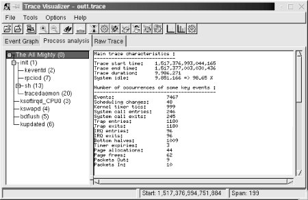
The system statistics start with a few numbers regarding the trace itself. In this case, the trace lasted almost 10 seconds and the system was idle for over 98% of that time. Next, the number of times a few key events have happened are provided. On 7467 events, LTT says that 1180 were traps and 96 were interrupts (with 96 IRQ entries and 96 IRQ exits.) This sort of information can help you pinpoint actual problems with the system’s overall behavior. The screen also displays a cumulative summary of the system calls made by the various applications running on the system.

As with the actual trace information, the statistics displayed in the “Process analysis” thumbnail can be dumped in text form to file from the command line. Look at the LTT documentation for more information on how this is done.

Sometimes the applications are not the root of performance degradation, but are rather suffering from the kernel’s own performance problems. In that case, it is necessary to use the right tools to identify the reasons for the kernel’s behavior.

There are quite a few tools for measuring the kernel’s performance. The most famous is probably LMbench (http://www.bitmover.com/lmbench/). LMbench, however, requires a C compiler and the Perl interpreter. It is therefore not well adapted for use in embedded systems. Another tool for measuring kernel performance is kernprof (http://oss.sgi.com/projects/kernprof/). Though it can generate output that can be fed to gprof, it involves the use of a kernel patch and works only for x86, ia64, sparc64, and mips64. As you can see, most embedded architectures are not supported by kernprof.

There remains the sample-based profiling functionality built into the kernel. This profiling system works by sampling the instruction pointer on every timer interrupt. It then increments a counter according to the instruction pointer. Over a long period of time, it is expected that the functions where the kernel spends the greatest amount of time will have a higher number of hits than other functions. Though this is a crude kernel profiling method, it is the best one available at this time for most embedded Linux systems.

To activate kernel profiling, you must use the profile= boot parameter. The number you provide as a parameter sets the number of bits by which the instruction pointer is shifted to the right before being used as an index into the sample table. The smaller the number, the higher the precision of the samples, but the more memory is necessary for the sample table. The value most often used is 2.

The sampling activity itself doesn’t slow the kernel down, because it only occurs at each clock tick and because the counter to increment is easily obtained from the value of the instruction pointer at the time of the timer interrupt.

Once you’ve booted a kernel to which you passed the profile= parameter, you will find a new entry in your target’s /proc directory, /proc/profile. The kernel’s sample table is exported to this /proc entry.

To read the profile samples available from /proc/profile, you must use the readprofile utility available as an independent package from http://sourceforge.net/projects/minilop/ or as part of the util-linux package from http://www.kernel.org/pub/linux/utils/util-linux/. In the following explanations, I will cover the independent package only since util-linux includes a lot more utilities than just readprofile. Download the readprofile package and extract it in your ${PRJROOT}/debug directory. Move to the package’s directory and compile the utility:

$ cd ${PRJROOT}/debug/readprofile-3.0
$ make CC=powerpc-uclibc-gcc

To compile the utility statically, add LDFLAGS="-static" to the make command line. The binary generated is fairly small. When statically linked with uClibc and stripped, for example, it is 30 KB in size.

Once readprofile is built, copy it to your target’s /usr/bin:

$ cp readprofile ${PRJROOT}/rootfs/usr/bin

For readprofile to operate adequately, you must also copy the appropriate System.map kernel map file to your target’s root filesystem:

$ cp ${PRJROOT}/images/System.map-2.4.18 ${PRJROOT}/rootfs/etc

With your target root filesystem ready, change the kernel boot parameters and add the profile=2 boot parameter. After the system boots, you can run readprofile:

# readprofile -m /etc/System.map-2.4.18 > profile.out

The profile.out file now contains the profiling information in text form. At any time, you can erase the sample table collected on your target by writing to your target’s /proc/profile:^[5]

# echo > /proc/profile

When done profiling, copy the profile.out file back to your host and have a look at its contents:

$ cat profile.out
               ...
    30 _ _save_flags_ptr_end             0.3000
    10 _ _sti                            0.1250
     8 _ _flush_page_to_ram              0.1053
     7 clear_page                       0.1750
     3 copy_page                        0.0500
     1 m8xx_mask_and_ack                0.0179
     2 iopa                             0.0263
     1 map_page                         0.0089
     ...
     1 do_xprt_transmit                 0.0010
     1 rpc_add_wait_queue               0.0035
     1 _ _rpc_sleep_on                   0.0016
     1 rpc_wake_up_next                 0.0068
     1 _ _rpc_execute                    0.0013
     2 rpciod_down                      0.0043
    15 exit_devpts_fs                   0.2885
 73678 total                            0.0618 0.04%

The left column indicates the number of samples taken at that location, followed by the name of the function where the sample was taken. The third column is a number that provides an approximation of the function’s load, which is calculated as a ratio between the number of ticks that occurred in the function and the function’s length. See the readprofile manpage included with the package for in-depth details about the utility’s output.

One of the most important metrics for real-time embedded systems is the time it takes for them to respond to outside events. Such systems, as I explained in Chapter 1, can cause catastrophic results if they do not respond in time.

There are a few known ad-hoc techniques for measuring a system’s response time to interrupts (more commonly known as interrupt latency). These measurement techniques can be roughly divided into two categories:

In the case of the self-contained method, you must write a small software driver that initiates and handles the interrupt. To initiate the interrupt, the driver does two things:

The driver’s interrupt handler, on the other hand, must do the following:

By subtracting the time at which the interrupt was triggered from the time at which the interrupt handler is invoked, you get a figure that is very close to the actual interrupt latency. The reason this figure is not the actual interrupt latency is that you are partly measuring the time it takes for do_gettimeofday( ) and other software to run. Have your driver repeat the operation a number of times to quantify the variations in interrupt latency.

To get a better measure of the interrupt latency using the self-contained method, plug an oscilloscope on the output pin toggled by your driver and observe the time it takes for it to be toggled. This number should be slightly smaller than that obtained using do_gettimeofday( ), because the execution of the first call to this function is not included in the oscilloscope output. To get an even better measure of the interrupt latency, remove the calls to do_gettimeofday( ) completely and use only the oscilloscope to measure the time between bit toggles.

Though the self-contained method is fine for simple measurements on systems that can actually trigger and handle interrupts simultaneously in this fashion, the induced method is usually the most trusted way to measure interrupt latency, and is closest to the way in which interrupts are actually delivered to the system. If you have a driver that has high latency and contains code that changes the interrupt mask, for example, the interrupt driver for the self-contained method may have to wait until the high latency driver finishes before it can even trigger interrupts. Since the delay for triggering interrupts isn’t measured, the self-contained method may fail to measure the worst-case impact of the high latency driver. The induced method, however, would not fail, since the interrupt’s trigger source does not depend on the system being measured.

The software driver for the induced method is much simpler to write than that for the self-contained method. Basically, your driver has to implement an interrupt handler to toggle the state of one of the system’s output pins. By plotting the system’s response along with the square wave generated by the frequency generator, you can measure the exact time it takes for the system to respond to interrupts. Instead of an oscilloscope, you could use a simple counter circuit that counts the difference between the interrupt trigger and the target’s response. The circuit would be reset by the interrupt trigger and would stop counting when receiving the target’s response. You could also use another system whose only task is to measure the time difference between the interrupt trigger and the target’s response.

However efficient the self-contained and the induced methods or any of their variants may be, Linux is not a real-time operating system. Hence, though you may observe steady interrupt latencies when the system is idle, Linux’s response time will vary greatly whenever its processing load increases. Simply increase your target’s processing load by typing ls -R / on your target while conducting interrupt latency tests and look at the flickering oscilloscope output to observe this effect.

One approach you may want to try is to measure interrupt latency while the system is at its peak load. This yields the maximum interrupt latency on your target. This latency may, however, be unacceptable for your application. If you need to have absolute bare-minimum bounded interrupt latency, you may want to consider using one of the real-time derivatives mentioned in Chapter 1.

Electric Fence is a library that replaces the C library’s memory allocation functions, such as malloc( ) and free( ), with equivalent functions that implement limit testing. It is, therefore, very effective at detecting out-of-bounds memory references. In essence, linking with the Electric Fence library will cause your applications to fault and dump core upon any out-of-bounds reference. By running your application within gdb, you can identify the faulty instruction immediately.

Electric Fence was written and continues to be maintained by Bruce Perens. It is available from http://perens.com/FreeSoftware/. Download the package and extract it in your ${PRJROOT}/debug directory. For my control module, for example, I used Electric Fence 2.1.

Move to the package’s directory for the rest of the installation:

$ cd ${PRJROOT}/debug/ElectricFence-2.1

Before you can compile Electric Fence for your target, you must edit the page.c source file and comment out the following code segment by adding #if 0 and #endif around it:

#if ( !defined(sgi) && !defined(_AIX) )
extern int           sys_nerr;
extern char *        sys_errlist[  ];
#endif

If you do not modify the code in this way, Electric Fence fails to compile. With the code changed, compile and install Electric Fence for your target:

$ make CC=powerpc-linux-gcc AR=powerpc-linux-ar
$ make LIB_INSTALL_DIR=${TARGET_PREFIX}/lib 
               > MAN_INSTALL_DIR=${TARGET_PREFIX}/man install

The Electric Fence library, libefence.a, which contains the memory allocation replacement functions, has now been installed in ${TARGET_PREFIX}/lib. To link your applications with Electric Fence, you must add the -lefence option to your linker’s command line. Here are the modifications I made to my command module’s Makefile:

CFLAGS        = -g -Wall
...
LDFLAGS       = -lefence

The -g option is necessary if you want gdb to be able to print out the line causing the problem. The Electric Fence library adds about 30 KB to your binary when compiled in and stripped. Once built, copy the binary to your target for execution as you would usually.

By running the program on the target, you get something similar to:

# command-daemon
 
  Electric Fence 2.0.5 Copyright (C) 1987-1998 Bruce Perens.
Segmentation fault (core dumped)

Since you can’t copy the core file back to the host for analysis, because it was generated on a system of a different architecture, start the gdb server on the target and connect to it from the host using the target gdb. As an example, here’s how I start my command daemon on the target for Electric Fence debugging:

# gdbserver 192.168.172.50:2345 command-daemon

And on the host I do:

$ powerpc-linux-gcc command-daemon
(gdb) target remote 192.168.172.10:2345
Remote debugging using 192.168.172.10:2345
0x10000074 in _start (  )
(gdb) continue
Continuing.
 
Program received signal SIGSEGV, Segmentation fault.
0x10000384 in main (argc=2, argv=0x7ffff794) at daemon.c:126
126             input_buf[input_index] = value_read;

In this case, the illegal reference was caused by an out-of-bounds write to an array at line 126 of file daemon.c. For more information on the use of Electric Fence, look at the ample manpage included in the package.

MEMWATCH replaces the usual memory allocation functions, such as malloc( ) and free( ), with versions that keep track of allocations. It is very effective at detecting memory leaks such as when you forget to free a memory region or when you try to free a memory region more than once. This is especially important in embedded systems, since there is no one to monitor the device to check that the various applications aren’t using up all the memory over time. MEMWATCH isn’t as efficient as Electric Fence, however, to detect pointers that go astray. It was unable, for example, to detect the faulty array write presented in the previous section.

MEMWATCH is available from its project site at http://www.linkdata.se/sourcecode.html. Download the package and extract it in your ${PRJROOT}/debug directory. MEMWATCH consists of a header and a C file, which must be compiled with your application. To use MEMWATCH, start by copying both files to your application’s source directory:

$ cd ${PRJROOT}/debug/memwatch-2.69
$ cp memwatch.c memwatch.h ${PRJROOT}/project/command-daemon

Modify the Makefile to add the new C file as part of the objects to compile and link. For my command daemon, for example, I used the following Makefile modifications:

CFLAGS        = -O2 -Wall -DMEMWATCH -DMW_STDIO
...
OBJS          = daemon.o memwatch.o

You must also add the MEMWATCH header to your source files:

#ifdef MEMWATCH
#include "memwatch.h"
#endif /* #ifdef MEMWATCH */

You can now cross-compile as you would usually. There are no special installation instructions for MEMWATCH. The memwatch.c and memwatch.h files add about 30 KB to your binary once built and stripped.

When the program runs, it generates a report on the behavior of the program, which it puts in the memwatch.log file in the directory where the binary runs. Here’s an excerpt of the memwatch.log generated by running my command daemon:

=  ==  ==  ==  ==  ==  == MEMWATCH 2.69 Copyright (C) 1992-1999 Johan Lindh =  ==  ==...
               ...
unfreed: <3> daemon.c(220), 60 bytes at 0x10023fe4          {FE FE FE ...
               ...
Memory usage statistics (global):
 N)umber of allocations made: 12
 L)argest memory usage      : 1600
 T)otal of all alloc(  ) calls: 4570
 U)nfreed bytes totals      : 60

The unfreed: line tells you which line in your source code allocated memory that was never freed later. In this case, 60 bytes are allocated at line 220 of daemon.c and are never freed. The T)otal of all alloc( ) calls: line indicates the total quantity of memory allocated throughout your program’s execution. In this case, the program allocated 4570 bytes in total.

Look at the FAQ, README, and USING files included in the package for more information on the use of MEMWATCH and the output it provides.