
Chapter 6. Stimulus Editor
Chapter Outline
6.1. Stimulus Editor Transient Sources84
6.2. User-generated Time–Voltage Waveforms91
6.3. Simulation Profiles91
6.4. Exercise92
The Stimulus Editor is a graphical tool to help you define transient analog and digital sources. The sourcestm library contains three source parts, shown in Figure 6.1, each of which provides the interface with the defined stimulus in the Stimulus Editor.
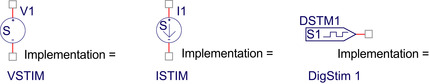
When you first place one of the sources from the sourcestm library, the implementation property is displayed in the schematic. This property refers to the name of the stimulus which is defined in the Stimulus Editor. Either you can enter a name of the stimulus on the schematic to start with, or you will be prompted for the stimulus name in the Stimulus Editor when started.
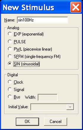
When the Stimulus Editor starts, the New Stimulus window will appear as shown in Figure 6.2. Note that the stimulus file name in 16.3 has taken on the name of the PSpice simulation profile, in this case, transient.stl. In previous versions, the stimulus name takes on the name of the project name.
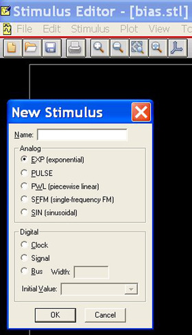
The New Stimulus window allows you to define analog and digital signals and prompts you to enter the stimulus name if you have not already defined the name in Capture.
6.1. Stimulus Editor Transient Sources
6.1.1. Exponential (Exp) Source
FIGURE 6.3 and FIGURE 6.4 show the two possible exponential waveforms which can be defined for a voltage or a current using VSTIM or ISTIM sources, respectively.
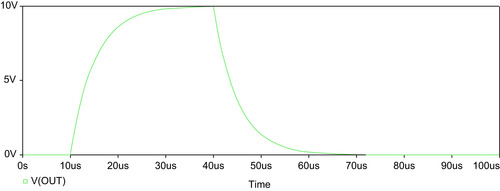
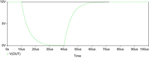
Both exponential waveforms start after a time delay (td1) and then exponentially rise or fall, using a time constant (tc1) between two voltages V1 and V2 up to a time td2. The waveform then decays or rises after td2, using a time constant (tc2).
For example, in Figure 6.3, the voltage is V1 (0V) up to td1 (10μs); then the voltage increases exponentially with a time constant given by tc1 (10μs) towards V2 (10V). The time for the exponential rise is defined by td2–td1 as 35μs (40–5μs), after which the voltage decreases exponentially with a time constant given by tc2 (5μs) back towards V1.
Figure 6.5 shows the attribute settings for the waveform in Figure 6.3, where:
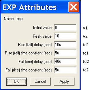
V1 – initial starting value at time 0s,
V2 – value that voltage rises or falls to,
td1 – start time (delay) of exponential rise (or fall),
tc1 – time constant of rising (or falling) waveform,
td2 – start time (delay) of exponential fall (or rise),
Figure 6.3 was defined using V1=0V, V2=10V, td1=10μs, tc1=5μs, td2=40μs and tc2=5μs.
Figure 6.4 was defined using V1=10V, V2=0V, td1=10μs, tc1=5μs, td2=40μs and tc2=5μs.
Now the exponential voltage is defined by:
6.1.2. Pulse Source
Figure 6.6 shows the definition for a voltage pulse waveform, where:
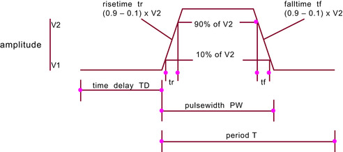
V1 – low voltage,
V2 – high voltage,
TD – the time delay before the pulse starts,
TR – rise time specified in seconds and is defined as the time between 90% and 10% of V2,
TF – fall time defined in seconds and is the time between 90% and 10% of V2,
PW – pulse width of the pulse,
PER – period of the pulse, i.e. the pulse frequency.
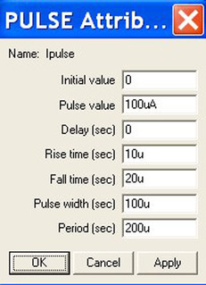
Similarly, current pulses can be defined using the ISTIM part as shown in Figure 6.7.
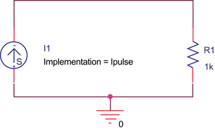
When you first place a VSTIM, ISTIM or DigSTIM part, the implementation property name and value are shown. You only need to display the name of the stimulus, so double click on the Implementation=, which will open up the Display Properties dialog box, and select Value Only (Figure 6.8).
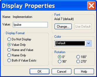
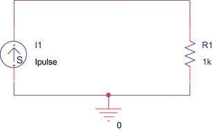
Figure 6.9 shows the ISTIM part with the defined current stimulus, Ipulse displayed. As before, to start the Stimulus Editor, rmb and select Stimulus Editor and then select PULSE for New Stimulus. Figure 6.10 shows the pulse attributes defined for a current pulse using the ISTIM part. The resulting current waveform is shown in Figure 6.11.
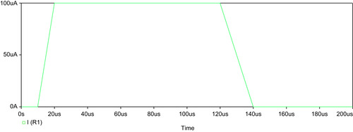 |
| FIGURE 6.11 Current pulse waveform using the attributes in Figure 6.7. |
6.1.3. VPWL
6.1.4. SIN (Sinusoidal)
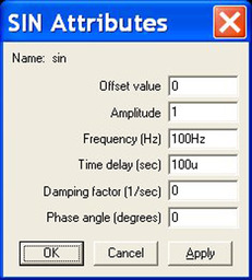
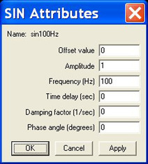
Figure 6.12 shows the attributes for a sinewave. The complete definition includes attributes for a damped sinewave, with a phase angle and an offset value. Offset value is the initial voltage or current at time 0s, Amplitude is the maximum voltage or current, Frequency (Hz) is the number of cycles per second, Time delay (s) is the start delay, Damping factor (1/s) is the exponential decay, and Phase angle (degrees) is the phase angle.
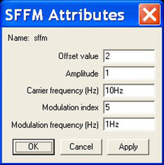
6.1.5. SSFM (Single-frequency FM)
This source generates frequency-modulated sinewaves as shown in Figure 6.14, which shows the modulation of a carrier frequency. The sinewave is given by:
6.2. User-generated Time–Voltage Waveforms
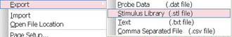
You can also use the waveforms generated by a transient analysis in Probe as a time–voltage source. In Probe, select File > Export, which gives the options shown in Figure 6.15.
An alternative method to create a time–voltage text file is to select the trace name in Probe, select copy and paste the data into a text file.
6.3. Simulation Profiles
Prior to version 16.3, when you launch the Stimulus Editor, a stimulus file with the name of the project is created; for example a project named stimulus will create a stimulus.stl. All the stimuli you create are saved in the stimulus.stl file and so in order to select a different stimulus, all you need to do in the schematic is to change the name shown on the VSTIM, ISTIM or DigSTIM source.
From version 16.3 onwards, the stimulus file is associated with the current active simulation profile and can be accessed via the simulation profile under the Configuration Files tab. In previous versions, there were separate tabs for Stimulus, Library and Include options.
Under configured files you will see the stimulus.stl file (see Figure 6.17). If you do not see the stimulus file then you can browse for the Filename. You can then add the stimulus file to the profile (Add to Profile). However, there are other options:
• Add as Global: all designs will have access to the stimulus file
• Add to Design: only the current design will have access.
Adding the stimulus file as Global is useful if you have created a standard set of stimuli to test all your circuits. You can add several stimulus files and arrange the order by clicking on the up and down arrows. The red cross deletes the selected file.
6.4. Exercise
NOTE
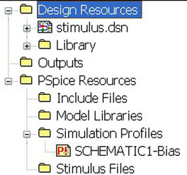
From release 16.3 onwards, there are some differences compared to previous versions. When you first create a new project in any release, a PSpice bias simulation profile is created by default. This can be seen in the Project Manager under PSpice Resource > Simulation Profiles. In order to keep compatibility between releases, delete the bias simulation profile in the Project Manager.
1. Create a project called stimulus.
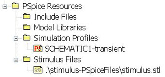
2. In the Project Manager, expand PSpice Resources > Simulation Profiles as shown in Figure 6.16 and delete the SCHEMATIC1-Bias profile.
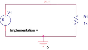
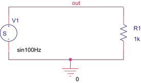
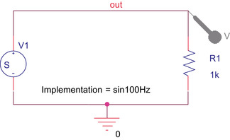
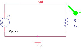
3. Draw the circuit diagram in Figure 6.17. The VSTIM source (V1) is from the Sourcestm library.
4. Highlight VSTIM and rmb > Edit PSpice Stimulus. In the New Stimulus window, name the source as sin100Hz and select a SIN source (Figure 6.18).
5. Create a 100Hz sinewave with no offset and amplitude of 1V. Leave all the other values at their default value of 0 (Figure 6.19). Click on OK and save the stimulus source and Update Schematic when prompted and exit the Stimulus Editor.
6. In Capture, the name of the stimulus is now shown on V1. Double click on Implementation= sin100Hz and select Value Only (Figure 6.20).
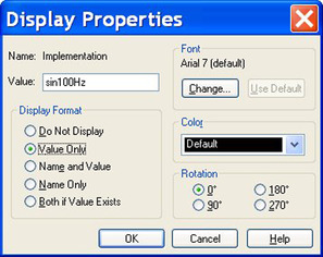
Only the name of the stimulus will be displayed, as seen in Figure 6.21.
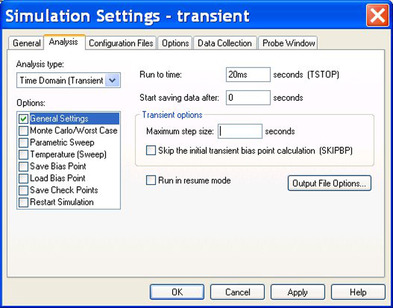
7. Create a PSpice simulation profile (PSpice > New Simulation Profile) and call it transient. In the Analysis type: pull-down menu, select Time Domain (Transient) and set the Run to time: to 20ms (Figure 6.22). Click on Apply but do not exit the profile.
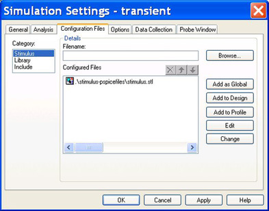
8. Select Configuration Files > Category > Stimulus and you should see the stimulus.stl file listed (Figure 6.23).
9. Place a voltage marker on node out (Figure 6.24), run the simulation (PSpice > Run) and confirm that a sinewave voltage appears across the resistor.
NOTE
If you see a flat voltage line in the Probe window, then you may have not deleted the default bias.stl file. See note at the beginning of the exercise. The Stimulus Editor was then invoked with the default bias.stl as the active simulation profile. If you do not see the stimulus file in the simulation profile (Figure 6.23) then Browse for the file, which can be found in the bias folder, and then select Add to Design.
10. In the Project Manager, expand PSpice > Resources > Stimulus Files and you should see the transient.stl stimulus file as shown in Figure 6.25. You can double click on the file here to open the Stimulus Editor to check the stimulus.
11. Highlight VSTIM in Capture and launch the Stimulus Editor. In the Stimulus Editor the previous SIN Attributes will be displayed. Click on Cancel.
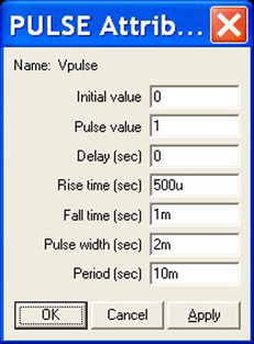
12. Create a pulse source named Vpulse (Stimulus > New) with an initial value of 0V, an amplitude of 1V, no initial delay, a rise time of 500μs, a fall time of 1ms, a pulse width of 2ms and a period of 10ms (Figure 6.26). Click on OK and save the stimulus but do not Update Schematic when prompted. Exit the Stimulus Editor.
NOTE
When entering attribute values, press the TAB button on the keyboard to move down to the next attribute box.
NOTE
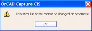
The stimulus is already named as sin100Hz in Capture and cannot be updated from the Stimulus Editor. In previous software releases, if you say yes to Update Schematic, the cursor will change to an hourglass and just sit there. You will need to switch to Capture, where you will see the dialog box in Figure 6.27. Just click on OK.
13. In Capture, double click on the stimulus name, sin100Hz, and change it to Vpulse as shown in Figure 6.28.
14. Run the simulation. PSpice > Run or click on the blue play button  .
.
15. Confirm that a voltage pulse waveform appears across the resistor.
16. In Capture, highlight VSTIM and rmb > EditStimulus Editor. In the Stimulus Editor the previous PULSE Attributes will be displayed. Click on Cancel.
17. Create a new stimulus, Stimulus > New. Name the stimulus Vin and select PWL (piecewise-linear).
NOTE
You may be asked if you want to change the axis settings.
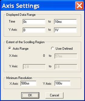
18. From the top toolbar, select Plot > Axis Setting. Set the waveform drawing resolution to that shown in Figure 6.29.
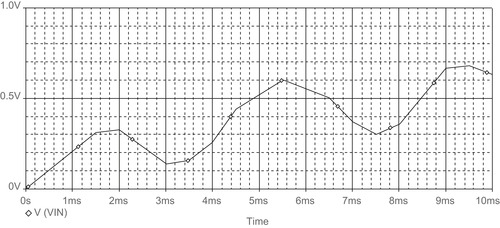
19. A pen cursor will appear. Draw a corresponding piecewise linear graph approximating the PWL voltage shown in Figure 6.30. The first point at (0,0) has already been selected. The accuracy does not matter as long as there are three peaks defined. This stimulus will be used in Chapter 7 on transient analysis. Press escape to exit draw mode.
20. If you want to delete or move a point, press escape out of draw mode and place the cursor on a point, which will turn red, and then delete or move the point. To return to draw mode, select Edit > Add or select the icon  or
or  .
.
NOTE
Prior to release 16.3, you can only place points forward in time; you cannot go backwards. If you want to delete or move a point, press escape out of draw mode and place the cursor on a point, which will turn red, and then delete or move the point.
21. Save the stimulus file and exit the Stimulus Editor but do not Update Schematic.
22. Change the name of the stimulus from Vpulse to Vin and simulate, and confirm that the piecewise voltage waveform appears across the resistor.
NOTE
The Vin source will be used in Chapter 7.
..................Content has been hidden....................
You can't read the all page of ebook, please click here login for view all page.