Keywords

Absolute and relative addressing; formula writing; basic formulas; error messages; error handling; novice; dynamic named ranges

Keep it simple stupid!

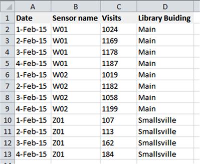
Excel formulas can scare many people. If you are one of those people, the thing to remember is your fear is based on an illusion. ALL formulas are very simple when broken down into their component parts. For example, say you have raw data for visits that looks something like the below. This is of course only a snippet, so pretend that you have years’ worth of data.

Chances are you would like to aggregate the data by Month and Year. The simplest way to do this is to add a column called “Year,” and another called “Month.” You should never ask the user to enter something that can be generated by a formula, and given you can calculate the month and the year from the date, you must use formulas. The formulas for Year and Month are very simple:

Month looks a bit different to Year for a reason. If you typed the formula=MONTH(A2) in the first row, you would get the number 1. If the date had been 7 Mar 15, then the formula would return the number 3. The MONTH() formula returns a number between 1 and 12, which represents the month of the year.

When it comes to pivot tables, for the most part you get out what you put in. So if you have months listed as numbers between 1 and 12, then when you aggregate the data by month, that is what you will see – i.e., numbers between 1 and 12. Some people may be fine with this, but a lot of people, including myself, would probably not like it. I prefer to see the months in their text form, preferably abbreviated to three letters, e.g., “Jan”, “Feb”, “Mar,” etc. It makes tables easier to read, and makes it instantly clear that the data refers to month, and not something else.

So, if you wanted to have the months displayed in text form, then there are many ways to do this. There will be the simplest way to write the formula, and an infinite number of more complex forms of the formula. The simplest way, I think, is the formula I have used above. What the TEXT formula does is take a value from a cell, and reformat it according to your specifications.

Paradoxically, it is actually pretty easy to write unnecessarily complex formulas, and here are two examples that will do the same as=TEXT(A2, “mmm”):

The measure of your talent as a formula writer is not whether you have produced something so complicated that it makes people stand back with fear, spontaneously put their hands over their mouths while whispering “oh my god!” You have failed if the next person taking over your role is reduced to adopting the fetal position upon realizing what they have inherited. A good formula is short, it is elegant, it does what it needs to do with the maximum clarity possible. Clearly, the above two formulas fail! They will return the correct results, but will require a lot more computing power to do it, and they will be difficult to change later given their purpose is so opaque. The first formula uses nested if statements to test if a certain number is present, then it return a corresponding month text value if true, otherwise if false it cascades down to the next if statement. There are so many nested if statements that this formula may not even work on earlier versions of Excel.

The second formula is shorter, but is still more complicated than it needs to be. Firstly, it requires you to create another table that defines the text value for each number value for a given month:

VLOOKUPs are very useful, and frequently unavoidable, and I will explain more about them shortly. However, avoid them if you can, as they can slow a spreadsheet down if it contains thousands of rows of data.

So, when you write a formula, unless you are very proficient with Excel, or it is blindingly obvious that the formula is as simple as it can be – you really should google what other functions are available that will do the trick. There are chat forums out there for every fetish, hobby, interest, and job imaginable. Whatever your question is, thousands of people have had the same question before, and at least half a dozen of them have submitted the question to an online forum. It will not take much effort to find useful information, you just have to look. Lucky you are a librarian, so you know how and where to look!

Make it easy stupid! Absolute and relative formulas

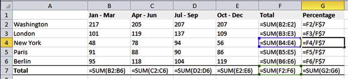
This is about making things easy on you. There are a number of ways to make your job a whole lot easier. The best and most frequent time saver you will ever use is the $ symbol in your formulas. When you write a formula, you can of course copy it to other cells, rather than retyping it every time. You can copy it to other cells by using the copy and paste method, or you can do it using the fill method. The fill method is the fastest way of copying formulas. To use this function, you simply select the cell that contains the formula you want to copy, and all the cells you want to copy the formulas to, then select either fill down, fill up, fill left, or fill right – depending on which direction you want to copy the formulas. For the sake of using an example, let’s say we have a library that for some reason has library buildings scattered in some of the world’s biggest cities. And for some reason you have ignored everything I have said about structuring raw data, and have decided to enter your data directly into a crosstab. In this instance you are counting the number of items loaned per quarter. And, yes, they are small numbers, but that is karma for bad data structure! Say you wanted to know the total for each location. That’s easy enough, just sum cells B2 to E2.

If you wanted to copy that formula down, for all the other locations, the easiest way to do this is to select cells F2 to F6, and select “Fill down” from the appropriate menu. I will not say where this menu is, because it changes with different versions of Excel. Alternatively, most versions of Excel have the same shortcut. If you press the Ctrl key, and the D key at the same time, it will fill down (Ctrl+D).

This is very simple, and most people will know how to do this. The next short cut is also very simple, but I have found a surprising number of staff that don’t use it.

When you fill a formula down, Excel will change the ranges in your formula to match what it thinks you want.

For example, when I used fill down on the highlighted range, Excel adjusted the row reference. So in row 3, the formula sums the values in row 3, not row 2. This is exactly what we wanted. For example, we would not want cell F3 to sum the values in row 2. However, there are times when this behavior is not helpful.

Say we wanted to create a percentage column. You could do this by entering the below formula in cell G2 (note, by setting the number format to percentage you don’t have to multiply the result by 100).

Now, if you select fill down (Ctrl+D), Excel will not do what you hoped for. See how the formula in G4 in the below image is dividing cell F4 by F9. Cell F4 is fine, but F9 is not. Excel has done this because when you fill down it simply increments the row and column references relative to the cell containing the formula.

There are a few ways to deal with this, including the good, the bad, and the ugly. The ugly way is to manually type in each formula. Don’t do that. The bad way, at least in this instance, would be to use a named range for cell F7 (i.e., the total). The good way is to use the $ sign in your formula.

The $ sign says to Excel, this is an absolute address, please don’t try to be clever when I fill my cells down (or up, etc.), just use the same reference point. In this example, we don’t want Excel to be clever with row 7. The solution, then is to put a $ sign in front of the 7, so as that your first formula in cell G2 looks like this: =F2/F$7. Now, when you select the cells you want to copy this formula to, and select fill down, Excel does what you want it to. All the formulas, from G2 to G6 now divide the row total by the grand total (i.e., cell F7).

Once you get the hang of when to use absolute addresses in your formulas (i.e., the $ sign), and when to use relative addressing (i.e., no $ sign), you will find that you can fill a spreadsheet with formulas very quickly and efficiently. On that note, you can toggle between relative and absolute addressing in formulas by using the F4 key, but you have to be editing the formula for this to work.

Formulas you must know

There are a few formulas that you absolutely must know. If you can count, add, subtract, and divide, then you will be fine. And if you can read, then you will be able to understand the logical formulas, such as IF, AND, OR. Even the most complex formula imaginable is simply a collection of these simple building blocks. Get to know these building blocks, and you will be fine.

SUM. This is an Excel classic, the go to formula that you will no doubt be visiting frequently. You can sum individual cells, or ranges. For example:

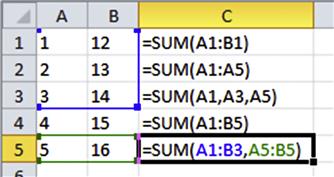
Notice there are five different examples of sum ranges. The formula in C1 sums across the columns, the next formula sums across the rows, the third sums a series of individual cells, the forth sums the whole block of numbers (A1 to B5) and the fifth formula sums two different blocks of cells. In other words, the sum function is very flexible, and this same flexibility applies to many formulas. The things you are summing do not have to be all grouped together.

COUNT. This formula counts the number of values in a range. It comes in four flavors: a formula that will only count cells containing numbers, and a formula that will count cells that contain anything, a formula that counts blanks, and a formula that will only count things under certain circumstances.

The above is reasonably self-explanatory, but if you are unsure, simply open up a spreadsheet, and type in the above. If you change the values in column A, e.g., delete the value in cell A1, you will see the formula returns a different result. Experimenting like this is a fantastic way to learn when you are unsure.

IF. This formula uses logic to test whether something is true or false, and then do one thing if it is true, and do a different thing if it is false. For example, if we wanted to have text to show whether Sally received more awards on average, then we might use the following formula:

The formula used in this example is: =IF(B1>B2, “Sally is above average,” “Sally is below average”). The formula structure for IF is: IF(logical test, value if true, value if false).

So, in this example, the first part of the formula is the logical test is “B1>B2.” In effect, this formula is asking “is this equation correct?” In this example B1=3, and B2=1. Therefore when those values are plugged into the equation, the result is 3>1. This statement is true, three is greater than one. Because the statement is true, the IF formula goes off and does the thing specified in the “value if true” section of the formula. In this example, the value if true is “Sally is above average.” If B2 contained the value 4, then the statement “3 is greater than 4” would be false. In this case, because the statement is false, the IF formula will return whatever you plugged into the “value if false” section of the formula.

However, what if both B1 and B2 contained 3? The formula would return “Sally is below average,” which is not correct. The formula would do this because the statement “3 is greater than 3” is incorrect, and therefore the formula would default to the “value if false” section of the formula. This means you need another IF statement in this formula, to deal with the possibility that B1=B2. To do this, you will need to create what is called “nested” IF statements. The formula will look like this:

The first part of the formula tests whether B1=B2. If this statement is true, then the formula will return “Sally is average.” If it is not true, then the formula will go to the “value if false” section of the formula. This section happens to be another IF formula, and hence the term nested IF statements. The “value if false” section of this equation is simply the first IF equation we discussed.

AND and OR. As librarians you will be very familiar with Boolean operators. You can use these in Excel too. The structure of AND and OR are the same, so for brevity I will simply refer to AND. The AND formula returns true or false, and is structured like this: AND(logical test 1, logical test 2, etc.).

This is probably not very helpful, so here is an example. Imagine you are considering buying an ice cream, and your decision was based on three things, is it hot, do I have time to eat it, and do I have spare change. Your AND formula would look like this: AND(is it hot, do I have time to eat, do I have spare change). If all those conditions are met, then the formula will return true; if even one of them is false (e.g., its not a hot day), then the formula will return false. This formula is particularly useful when used in conjunction with the IF statement. For example IF(AND(is it hot, do I have time to eat, do I have spare change), buy an ice cream [value if true section of IF formula], do not buy an ice cream [value if false section of IF formula]). Of course this is a silly formula that you could not actually plug into Excel, but the structure is the same. Here is a real example.

The formula is: =IF (AND(F3>1, F4>0),“Yes”, “No”). The first part of the formula is the logical test, which in this case is an AND statement. If the AND statement returns true, then the IF formula will go to the “value if true” section of the formula, which happens to contain the value “Yes.” If the AND statement returns false, then the IF formula will go to the section dealing with “value if false,” which in this example contains the value “No.” In this example the AND statement is essentially asking, did Sally get more than one librarian of the Year award, and at least one other award. If this is true, then she is a superstar, if not, then she is not a superstar.

COUNTIF. This formula is a little bit more complicated than COUNT, but not by much. COUNTIF comes in two flavors: the simple version; and the extended version.

In the first formula, the COUNTIF statement looks through the range B2 to B19, and counts the number of entries that are equal to “Sally Smith.” The second formula does the same thing, but instead of typing in “Sally Smith,” I have pointed the formula to the value in cell E3, which happens to be “Sally Smith.” If I pointed it to cell B4, the formula would have returned an answer of 1, as there is only one “Ellie Vader” in the list.

The formulas in cells G2 and G3 have the same structure, its just a slightly different way of doing things. Usually, its better to refer to a cell, than to plug the actual value into a formula. This is because if I changed the spelling of “Sally Smith” to “Sally Smyth,” then I would need to update the formula, as well as all the cells.

The third formula uses COUNTIFS, and is only available in more recent versions of Excel. It has the same functionality as the above formula, with the only difference being that you can run multiple criteria. In the above example, Sally received four awards all up, of which three were “Librarian of the Year,” and one was the “Innovation Award.” If you wanted to count the number of times Sally received the Librarian of the Year award, then you would need to use the COUNTIFS formula.

The formula is=COUNTIFS(B2:B19, H4, A2:A19, I4).

If you find that too confusing, then refer to this formula instead:=COUNTIFS(B2:B19, “Sally Smith,” A2:A19, “Librarian of the Year”).

The first part of this formula starts of the same as the regular COUNTIF formula – i.e., the formula looks through the list of names and counts the number of times it finds the name “Sally Smith.” The second part of the formula (i.e., …A2:A19, “Librarian of the Year”) looks through the range A2 to A19, and counts the number of “Librarian of the Year” entries. The formula then only returns those rows where both those criteria are satisfied. There are only three rows where the Staff Name is “Sally Smith,” and the Award Name is “Librarian of the Year,” so the formula returns 3.

If you have Excel 2003, and need this formula, don’t panic. There is almost always more than one way to do something in Excel. For example, you could use SUMPRODUCT:

The formula SUMPRODUCT might look a bit intimidating at first, but its not that bad. The formula I used was:

=SUMPRODUCT(--(A2:A19=F4), --(B2:B19=E4))

Alternatively, if you find “=F4” and “=E4” confusing, refer to this formula instead:

=SUMPRODUCT(--(A2:A19=“Librarian of the Year”), --(B2:B19=“Sally Smith”))

SUMPRODUCT sums the values in a range (array), depending upon the criteria you applied. Just like the COUNTIFS formula, you can use multiple criteria. The double -- after the first bracket forces Excel to treat true and false as 1 and 0. So what the hell does this mean?? Well, the first part of the formula looks in the range (array) A2 to A19 for any cell that contains “Librarian of the Year” (remember, F4 contains the text “Librarian of the Year,” we could have used that text instead of F4 if we wanted). Now, every time that the formula finds “Librarian of the Year” it returns a value of TRUE. So, its just like you running your finger down the list and asking, is that a Librarian of the Year award, and then answering true or false, depending upon what is actually in the cell. You cannot add up TRUEs, so putting the “--” in the formula forces Excel to convert all the trues to 1s and falses to 0. So, imagine now you are running your finger down the list of awards, and every time you see “Librarian of the Year” you write down 1. If you summed all those 1s up, you would get 15, and this is exactly what this formula would return if it stopped at that point. However, there is a second part to the formula “--(B2:B19=E4).” This second part of the formula follows the same logic as the first part. If you were to do this manually, you would scan your finger down the list of staff names, and every time you found Sally Smith you would add 1 to your note pad. If you were only counting Sally Smiths you would get 4. But you are not. The formula is counting each row where the award is “Librarian of the Year” AND the recipient is “Sally Smith.” There are only three rows that fit that criteria, so hence the answer is 3.

As I said previously, there are always more ways to do things in Excel, though some are unnecessarily complex. Here is another way to count the number of times Sally Smith won the “Librarian of the Year” award. The following example is probably too complex in this context:

In this example, I added a field called “Concatenation,” which is a fancy word for join, in column D. Under this heading I added a formula that combined the text of “Award Name” with “Staff Name” into a single cell. I then used COUNTIF to count the number of rows in column D that contained the text “Librarian of the YearSally Smith.”

CONCATENATE. Even though the above formulas are unnecessary, as there is a much simpler formula available for the required job, there are times when you will need to create a combined key, or simply join values. Say you have a list of first names, and surnames, and you wanted the full name. You can do this one of two ways:

Both the formulas in columns C and D return the same result. I prefer the formula in column C, because its shorter. But that is just a personal preference.

SUMIF. The best way to think of SUMIF is as a COUNTIF that sums up the values, rather than count them. However, if you have skipped COUNTIF, or are still struggling a bit with it, you probably would be annoyed with me referring you back to COUNTIF. So, here is a SUMIF example.

There are two versions of the SUMIF formula here, and both are doing the same job, they are just structured slightly differently. SUMIF adds all the values in a specified range, but only if the cells in corresponding range meet your criteria. For example, say you wanted to total up all the visits to the main library, and you wanted to do this manually. You would scan your eye down column D, and every time you saw the word “Main,” you would look at the corresponding row in column C, and write down that number on a separate piece of paper. Then once you have finished scanning the list, you would get your piece of paper, and add up all the numbers. SUMIF is doing the same thing. In the first example (the formula in cell G3), SUMIF looks through the range D:D, and looks for the word “Main.” When the formula finds the word “Main,” it looks across to corresponding row in column C, and adds that to a running total. So, when the formula looks at cell D2, it sees that the contents of the cell is “Main,” so it takes the number 1024 in cell C2, and adds it to a running total.

The syntax for the SUMIF formula is: SUMIF(range, criteria, sum range). So the first part of the formula points to the range containing your criteria (e.g., the Library Building name in column D). The second part of the formula, “criteria,” specifies the criteria you wish to apply, e.g., we are only interested in the “Main” library. The last part of the formula, “sum range,” points to the range that contains the values you want to sum when your criteria are meet, which in this case is column C.

VLOOKUP. If SUM is the bread of Excel formulas, then VLOOKUP is the butter. They are unavoidable, and you will have to use them at some point in your formula writing career. The VLOOKUP formula is like the index in a book, it helps you to find something. Imagine you had a spreadsheet that contained the number of library visits, and that you populated this spreadsheet by exporting data from your gate sensor software. Imagine that you were able to export three fields, the date, the sensor name and the number of visits. Each senor has a unique name. You have two entry gates for your Main Library, and the sensors for these are named W01 and W02. You also have a smaller satellite library located, naturally enough, in the quiet suburb called “Smallsville.” The sensor at Smallsville is called “Z01.”

When you are asked to report on the number of visits, you are not going to report how many visits there were for W01, W02, and Z01. Your audience would be confused, and even if they did understand what the codes meant, they would most likely not be interested in your data being broken down by the two sensors for the Main Library. Chances are they are only going to want to know how many visits there were by location at best. If we are using pivot tables, and we absolutely should be (discussed in Chapter 7), then you must also have another column that summarizes the sensor names by library building. You could do this manually, i.e., type in the library building for each and every record:

Here there are only 13 rows of data, so its not such a big job. However, if you have tens of thousands of rows of data, which is quite probable if you can export your data by the hour, then no sane person would suggest you type this in manually. This is where VLOOKUP steps in. If W01 always represented the main library, W02 always represented the main library, and Z01 always represented Smallsville, then wouldn’t it be wonderful if there was a formula that we could use to look up this value in a table, and tell us what library building the sensor belongs to. This is what VLOOKUP does. Below is our lookup table for the job, it tells us the name of each gate sensor, and the library building the sensor is located in.

All the VLOOKUP formula needs to do then is to use the sensor name in our main table, and return the corresponding Library Building name. It’s a bit like being given a key to a post office box. Once you have the post office box number, you can go off and retrieve the contents of the post office box.

This is the formula:=VLOOKUP(B2, G2:H4, 2, false). The syntax for VLOOKUP is:

VLOOKUP(lookup value, table array, column index number, [range lookup – i.e., approximate or exact match]).

Here is how it works. The first part of the formula, “B2,” is the value you are looking up. If you look in cell B2, you will see that the value being looked up is “W01.” “W01” is the equivalent of your post office box number. The second part of the formula “G2:H4”, says “here is where you are looking for the data”. This is the equivalent of the Post Office address. The third part of the formula, “2” says “what we are looking for is in the second column.” The second column of what? The second column of the range you told it to look in, i.e., G2:H4. Therefore, column H is the second column. Finally the last part of the formula “false,” says “only return something that matches the lookup value (‘W01’) exactly.” So, this formula is looking for “W01” in column G, and if it finds and exact match, which it does, return the corresponding value in the second column of the lookup table (column H). So the formula in D2 returns “Main.”

If you are still struggling with this, imagine you had to manually enter the library building into the spreadsheet. You would look at the sensor name, scan your eyes across to the sensor table, look for W01 in that table, and then when you found it, you would know what library building the sensor was located in by scanning your eyes across to the cell on the right. The VLOOKUP formula is doing exactly the same thing.

You might notice that VLOOKUP does not specify which column in the range G2:H4 to look for “W01.” This is because VLOOKUP always looks in the first column of the “table array,” which in this case is column G. So if you swapped columns G and H around, the formula would no longer work.

The lookup table can be located anywhere, on any worksheet, or even in another workbook (not advised!). In this case I have put the lookup table on the same sheet in range G2 to H4, so you can see it easily. Normally, however, you would put it on another sheet. Notice I have used relative addressing in the above formula, which means when I fill it down to row 13, only the first formula will have the correct address for the lookup table. Try copying this example, and filling the formula in cell D2 down to D13, you will see what I mean. The simple answer is to use absolute addressing for the lookup table by using the $ sign as follows:=VLOOKUP(B2, $G$2:$H$4, 2, FALSE). This will ensure that as you paste the formula down, it will keep pointing correctly to the lookup table, which does not move.

HLOOKUP. This formula is like the poor neglected cousin of VLOOKUP, except in this case, you probably should keep HLOOKUP locked up in the attic, and only let out in the sun on the rare occasion. The best way to imagine HLOOKUP, is to understand VLOOKUP, then rotate your head 90° to the horizontal position. It does exactly the same as VLOOKUP, but only horizontally. The reason I say you should use it very rarely is because if you have structured your tables correctly, they will be in columns, and therefore any lookups you require will be in the vertical, not the horizontal axis.

Named ranges. These are a fantastic tool for making your spreadsheet easier to understand and manage. When you write a formula, you can address the cell directly, use indirect referencing, or use a named range. For example, with the visits spreadsheet, we could put the sensor lookup table on a new sheet, define the lookup table as a named range, then you could use that named range in the VLOOKUP formula. There is a chance that did not make much sense, so here is the step-by-step version. If you have not already done so, go back and read the VLOOKUP formula above before reading on.

Firstly, put your lookup tables on a sheet called “Validation.” Next, you will need to use the name manager. This will be located in different places, depending upon the version of Excel you are running. So, you might have to do a little detective work via the built-in help or Google to find it. Once you have found how to activate the name manager, the next step it is to use it. Highlight the lookup table (G6 to I8 below), then call it a sensible name. A sensible name is one that will make sense in the formula, i.e., it is brief and reasonably self-explanatory.

I have called this range “SensorLookup.” Notice how Excel defaults to using absolute addresses (the $ signs) for the address. This is good; we want it to be absolute. The named ranges have a horrible habit of radically shifting position when you add and delete columns and/or rows. Using absolute addresses (i.e., using the $ symbol), stops this behavior. So if it is not an absolute address, make it one. When you click OK, you will now have a new named range called “SensorLookup.” You can type this in the same way you would have previously used the range “G6:I8”. For example, if you wanted to simplify your previous formula for looking up the building a sensor is located in, you could now change your formula to:=VLOOKUP(B2, SensorLookup, 2, FALSE)

Not only is this tidier and easier to read, but it also has other advantages. If your library expands, and you open a new building, you only have to remember to update the sensor lookup table, and ensure that the named range is updated accordingly. Any formula that refers to the SensorLookup named range would be automatically updated. So it also makes managing the data easier.

This is the vanilla version. You can also use a dynamic named range, one that will automatically expand and contract when you add or delete new values to a list. That way, if you need to add values to a lookup table, you do not even need to worry about updating the named range – as it will happen automatically.

Dynamic named ranges. When you go to edit a named range, and you click on the formula, it will highlight the cells to which the named range refers. This is a good way for checking whether your named range is actually pointing to the right cells. If the dashed line is not highlighting what you expected, then you need to adjust your formula. I have used a dynamic named range in the below screenshot. If I added a new sensor into row 9, the formula would automatically expand to accommodate the new data.

Here is the formula and how it works:

=OFFSET(Validation!$G$6,0,0, COUNTA (Validation!$G$6:$G$600), 2)

The OFFSET function returns a cell or range from another place in the workbook. This will not make much sense at the first, so just continue to plough through for a bit longer.

The OFFSET formula structure is OFFSET(reference, rows, columns, [height], [width]). Wherever you see [ ] in Excel, that means these values (arguments) are optional – i.e., you could end the formula at “columns”.

The first part of the formula, the “reference” section, is your starting point. In our case the starting point is cell G6. This is because regardless of how many sensors I add to the list, the first sensor in this particular sheet will always be located in cell G6. Therefore that is our starting point. The word “Validation!” in front of G6 is simply the name of the worksheet. Since we are working across several worksheets, we need to know which sheet we are pointing to. The next part of the formula is the number of rows and columns we want to offset. In this instance, we don’t want to use those functions, so we plug in zero for rows, and zero for columns. If we plugged in a value of one for rows and one for columns, the range would not start at G6, it would start at H7. And this is not what we want in this case. See how plugging a 1 into the rows and columns moved the dashed line across so as that the starting point is now at H7. The dashed line covers the range that our formula refers to, and while in some situations we might want to offset our range by a certain number of rows and columns, this is not one of them. Consequently, I have plugged zero into the row and column values for the formula.

What we do want to do, however, is make the formula refer to a range that will cover all the sensors we might wish to add to the list. The last part of the formula, the 2 at the end, is the easiest. We will always have two columns for this data, the “Sensor Name,” and the “Library Building.” Consequently, the range width will always be 2. The last part of the formula refers to the cell width: OFFSET(reference, rows, columns, [height], [width]), so that is why the number 2 is at the end. The [height] section of the formula is the most tricky, as this will change as we add or delete sensors to the list. The best way to know how many values there are in the list is to count them, and that is exactly what I have done. COUNTA counts all the cells that are not blank within a specified range. I have asked the formula to count all the non-blank cells between G6 and G600. I chose G6 as the starting point, as there should always be a value in G6. The reason I selected G600, however, was arbitrary. I could not count the cells between G6 and G7, because in this example there is a value in A8. If I did this, the formula would not capture the full range, as there are only two non-blank cells between G6 and G7, but there are three rows of data. Consequently I picked 600, because I thought the list would never extend beyond the row 600, so it was pretty safe to count non-blanks between the range G6 to G600. If your list ever did grow past row 600, then you would need to change this formula. So always try to imagine the most outrageous list possible, then double it to be safe.

As you can see, a formula that looks quite complex is actually very simple when broken down into its component parts. Using a dynamic named range may seem like a lot of unnecessary work, but I assure you, that is not the case. A good spreadsheet is robust and flexible. You will inevitably change lookups and validation lists, and if you don’t ensure that your named ranges are automatically capturing these changes, then you will have to do this manually. This will be a big job if you have a lot of lookups and validation lists. Worse still, if the ranges for lookups and validations are not automatically adjusted, then when you update those lists, there is a good chance you will forget to update the static ranges your lists are using. The amount of time it takes to create dynamic named ranges is only marginally longer than it takes to make a static one, and the first time you have to update the list, those seconds you saved by using a static list will be immediately lost. So don’t be lazy, keep re-reading this section on dynamic named ranges until you understand them, then use them.

Typical error messages and what they mean

At some point in your formula writing career, Excel is going to give you some cryptic looking error messages. It is important that you know why you have an error, if you wish to address that error.

Here are the error messages you are most likely to encounter, and what they mean

Managing error messages

There are situations where it might be impossible to avoid an error, but you don’t want users to see an ugly error message that might just confuse and worry them. So long as you know exactly why you are getting the error message, and in that context it is perfectly OK to ignore the error, then you can use a formula to do something different if an error is found. For example, say you wanted to allow users to add new sensor codes to the raw data sheet for visits, but you also wanted to let the user know if they have added a code that is not in your lookup table. You could do something like this:

And this is what the formula returns:

You might not like that error message, no big deal, you change it to whatever you want, like say “unknown.”

The formula is: =IFERROR(VLOOKUP(B2, SensorLookup, 2, FALSE), B2&“not found in Sensor Lookup table”).

This formula looks long, because it is joining two different formulas. However, if you look at each formula in isolation, it will be much easier to understand. The formula structure for IFERROR is: IFERROR(value, value if error). The IFERROR formula is doing two things, it tests whether an error exists, and if one does not, then it will run whatever formula or value you plug into the first section of the formula (i.e., the “value” section). If there is an error, the formula will return whatever formula or value you plug into the second section of the formula (i.e., the “value if error” section). So in the above formula the first section is running the VLOOKUP formula (see the VLOOKUP example earlier on). If all goes well, and the VLOOKUP does not return an error, then the IFERROR formula will return the results for that VLOOKUP. However, if the VLOOKUP does result in an error, then the IFERROR formula will return the formula or value specified in the second part of the IFERROR formula. So, in row 2, VLOOKUP returns an error, as the value “Q” does not exist in the sensor lookup table. IFERROR then says, well this formula has an error, so I will follow the alternative set of instructions given to me in the second part of the IFERROR formula, which might be something as simple as returning the word “unknown.” I used a formula for the error message, to show that it could be a formula – but it could be straight text. The formula I used was to look in the cell B2, and join whatever you find there to the text “not found in Sensor Lookup table.”

IFERROR is not available in all versions of Excel, though there are other similar formulas available that with a little extra work will do the trick. For example, ISERROR will return true for certain errors, so you could test if the error exists using an IF statement, and if the error is not present do the formula, and if there is an error, then throw up a warning message.