
Stop, police!
This chapter explains why it is important to make robust user proof spreadsheets, and how to create spreadsheets that users cannot break. Readers are encouraged to think beyond their own needs for spreadsheets, and to consider the change in approach that is required when creating spreadsheets for wider distribution. There are a number of tools available to maximize data integrity, including data validation, hiding data, tables, and limiting what uses can do with cells. These tools are explained in simple step-by-step terms, using library specific examples. For the readers that are interested in stretching themselves, this chapter also explains the use value of dependent lookups, and explains in detail how these formulas work.
Keywords
Data protection; data validation; tables; dependent lookups; bullet proof spreadsheets
If a user can stuff up your spreadsheet, then chances are they will. By and large they will not do this intentionally, but that does not matter. If you do not place boundaries on how staff can use your spreadsheets, they will soon render them useless. With all the effort you are spending on collecting the data, you want to ensure that when it comes time to using the data that it is as accurate and up-to-date as it possibly can be. The bottom line is, data integrity is everything. Without data integrity, all you have is a heap of rubbish numbers. So if you are going to bother collecting the data, then you should do all of the following:
• Store your spreadsheets on a server that is automatically backed up on a daily basis. In most cases your corporate file servers will be backed up, but check if you are unsure.
• Use the workbook, sheet, and cell protection functionality to ensure that staff can only change those parts of your spreadsheets that you want them to change.
• Use data validation wherever possible to ensure that staff can only enter values within a range or from an approved list.
• Create policies and procedures to ensure that data is updated at regular time intervals, and data cannot be retrospectively entered prior to that date.
Protecting data
There are a few levels of protection that apply to spreadsheets:
• You can require users to enter a password to open and/or modify the workbook. You can access this via the “Save as” menu. Look under “Tools”>“General options” on the “Save as” dialog box. Obviously, you should ensure the password is recorded somewhere safe that a few key staff can access. It is highly unlikely that you will need to apply this level of protection, because if you don’t want someone else to see something, the simplest solution is to save it to a place that only authorized staff can access.
• You can stop users from moving, hiding, un-hiding, deleting or renaming worksheets by clicking on the “Protect Workbook” icon, and ticking “Protect workbook for structure.” You should protect any workbook that will be used by multiple staff. You should also enter a password, because it only takes one person to realize they can do away with the annoying straightjacket you have put on them by simply clicking again on “Unprotect Workbook,” and then before you know it, everyone knows, and like a bunch of inquisitive gibbons they all start clicking away the protection, and unconsciously vandalizing your workbooks. Not good!
• Excel allows you to control many aspects of what users can and cannot do with a worksheet. When you click on “Protect Sheet,” you will get the following options:
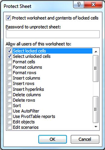
I am very draconian, and I usually only allow users to select unlocked cells, and use pivot tables. This has turned out to be a very good policy, and one I strongly recommend you go with. When you protect a sheet, the same deal applies. If you don’t use a password, then you will soon find that staff will just unprotect your sheet.
If you only want users to select unlocked cells, then you will need to define which cells are locked, and which are not. You will also need to protect the sheet. Anyone can do anything with a locked cell if the sheet has not been protected.
There are several ways to lock a cell. Most versions of Excel will allow you to right click a cell, select “Format Cells,” then select the “Protection” tab on the “Format Cells” dialogue box. Then you tick or untick the “Locked” checkbox.
Setting up your cell protection is simple if you have organized your data according to the structure outlined in Chapter 5.
• The first step is to make sure all the cells are locked. Click on the square in the top left hand corner of the Excel grid. This action will select all cells. Next, open up the Format Cells dialogue, and select locked. Doing this locks every single cell on the sheet.
• Step two is to unlock all the columns that you are happy for your staff to enter data into. Select all the columns of data under which you are happy for staff to enter data. Don’t worry at this point that your selection will include headers. Open Format Cells dialogue, then uncheck the locked check box.
• The final step is to lock the cells above the header. Select every row down to and including the header row, open the Format Cells dialogue, then select locked.

After those three steps you need to protect the sheet. Once this is done, in this example, the only cells that staff will be able to edit are those between columns B and E for rows 11 onwards In this example the formulas are completely safe, the title and the column headers are also completely safe. If you have used data validation, the risk of invalid data will be greatly reduced. You should hide anything the users does not need to see, which in this example is column A, and columns F through to L. This will provide staff with a very clean and easy to use data entry screen.
Data validation
It is still possible for users to muck up your spreadsheet even after you have locked down all the appropriate cells, and protected the workbook and all the worksheets.
A spreadsheet will be useless if users cannot enter data, but if they are allowed to enter the first thing that comes into their head, then you will end up with the following sort of problems:
• Variables that are described and/or spelled many different ways. For example, if you have a spreadsheet to record information literacy classes, and a field to describe the topic taught, the variety of descriptions for a lesson on Boolean searching might include: searching, searches, search, Boolean, Searching Boolean, Boolean searching, Boolean searches, navigating library discovery layer, etc. When you try to run a pivot table containing the distribution of attendances by topics, you are going to get a new row for each and every way your users describe the same topic.
• Users will enter invalid data. For example, say you were running a series of book reading classes for children, and you asked the facilitator to provide feedback on things such as the children’s reaction. You might have a specific list of responses you are interested in, such as unfocused, listening intently, actively engaged. If you left the “Behavioral response” field a free text column, you will get a wide variety of responses that do not offer useful information, such as “one child left early.”
• Data that is incorrectly entered, leading to formula errors. For example, someone might enter a date that does not exist, such as 33 Jan 2015. Any formulas that refer to that date will return an error. A user might put text in a cell where a number is expected. For example they might enter the number of visits as “nil,” instead of 0. This will also create errors.
Applying data validation rules to cells will mean that users can only enter certain values. For example, you can provide users with a drop down box that has a list of values, and stop them entering anything other than what is in that list. You can force users to enter a number within a range. For example, you might only allow users to enter a number between 20 and 100. You can also force users to enter a valid date, and specify that the date they enter is between two dates. For example, you can specify that users can only enter a valid date between 1 Jan 15 and 31 Dec 15. There are a few other options, but you should get the idea by now. To put it succinctly, the purpose of using data validation is to ensure that users enter values in the way you expect them to be entered.
Applying data validation rules is very simple, and there are two ways to do it. “Hardwire” it into the cell, or refer to a list. You should avoid hardwiring data validation lists, unless you are absolutely sure that the values will not change. You can change hardwired lists, it is just fiddly, and because you have to open the validation rules dialogue box to be able to see the validation rules, it can make maintenance of validation lists much more labor intensive than it needs to be. If you have to hardwire the list, you just type the values directly into the validation list dialogue box. For example, for lists choose “list” as a validation type in the validation dialogue box, and then just type in the values, separating each one with a comma, e.g., Jan, Feb, Mar, Apr, May, Jun, Jul, Aug, Sep, Oct, Nov, Dec. In Excel 2010, the data validation menu is on the Data tab on the Excel main menu.
When you are applying data validation to your raw data sheet, the easiest and most effective way to do it is to apply it to the entire column. Once you have finished applying data validation to each column, you can then remove the data validation from the title and headers by selecting rows 1 to 10 in the below example, then open the data validation dialogue box, and selecting “any value.” You only need to do this if you have to edit the headers or title, otherwise, you can just leave rows 1 to 10 as is.
Here is a screenshot showing how you could force users to enter a valid date between 1 Jan 15 and 31 Dec 15:
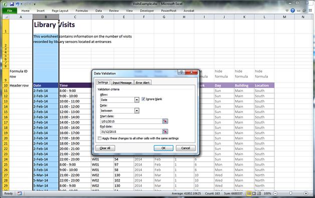
Note that you can type the start and end dates directly in to the Data Validation dialogue box, or you can click on the “select cell” icon on the right hand side of the text box, and point to a specific cell that will contain the start date, and another to contain the end date. This can be useful if you wanted to set your spreadsheet on autopilot. For example, you could point to a cell that contains a formula that makes the start date 30 days before the current day.

If you pointed the start date in the Data Validation dialogue box to cell $C$6, and the end date to cell $C$7, then the users will only be able to enter a date sometime between 30 days ago, and tomorrow. If you want to use more static start and end dates, then it would still be worth pointing to a cell value, that way you can update all your data validation lists in one place, i.e., the “Validation” sheet.
You may have noticed when you tried using data validation that there are also some other options, including options for specifying input messages, and error alerts. You can use the title and input message to make the data entry a little more user friendly. This is probably of questionable value, but you may find some use in some situations.
The more useful function is the “Error Alert.” Using this function you can apply one of three rules. You can stop the user from entering the value, you can give them a warning (which they can ignore), or you can simply provide information. The last two are pretty much the same, they both give the user the option to ignore the data validation rules.

In most cases you are probably going to want to apply the stop rule. However, there might be cases where it is worth being a bit more flexible. For example, staff at your information desk may be required to record the main topic of support they provided. For the most part, the staff might just pick an item from a list. However, you might want to capture the occasional request that does not fall within a predefined list, and allow staff to enter something new after you gave them a warning. This is a good compromise between managing data integrity, and ensuring that you are still able to capture changes in trends. If you are finding that you are getting a lot of new queries, for example, then that in itself will provide you with valuable information that you can use to fine tune your service through training staff to meet these new emerging needs. After a while, you might expand the validation list for the information desk to include these new topics.
While on the topic of lists, the best way to make it easy to manage your validation lists simple is to put them all on the one sheet, and use either a dynamic named range to point to the relevant list, or a table. For example, if you wanted to limit the sensors staff could enter into your visits spreadsheet, then you could do this by creating a dynamic named range called “SensorNameList” (for help with named ranges see previous chapter). The next step is to open the “Data Validation” dialogue box, select “List” from the “Allow” drop down box, then type in “=SensorNameList,” without the quotation marks of course!

If you have done this correctly, any new sensor you add to your validation list will appear as a new option in your drop down list for sensors.
Dynamic named ranges can scare people, they don’t work with dependent lookups, they can start to become a bit unnecessarily complex when using them to drive validation lists (as you might end up with a lot of them), and sorting them can be a little bit fiddly. There is a much better option; using tables. However, I haven’t put you through dynamic named ranges just for my own sadistic pleasure, there are many times when you will still need to use them. When it comes to validation lists, however, tables are far superior method for populating validation lists, as they allow you to sort the lists easily.
Using tables
Excel has a function that allows you to convert a range of data into a table. Once a range has been converted to a table, you can easily sort and filter the data by any of your fields. The table automatically expands as you add new rows of data, and when you do this, the table will automatically add any formulas you have in your table to the new row. Finally, you don’t have to worry about dynamic named ranges, as any validation list that refers correctly to a table will automatically expand and contract as new data is added or deleted from the table.
Tables sound great, and they are, but there is a good reason for not converting everything to a table. If you use a table, you cannot protect the cells. Well, strictly speaking you can, but that then means the table acts like a range, i.e., you cannot add and delete rows, effectively rendering the table useless as a table. One possible workaround is to not protect your sheet, use validation lists in all the visible columns, and hide any column with a formula. This is quite risky, as there is nothing to stop users changing the field names (which will have an impact on any pivots running off the table), and there is nothing to stop users from deleting formulas accidently from your hidden columns. For these reasons I strongly recommend that you do not use tables for your raw data, at least until Microsoft addresses this Achilles heel for tables.
However, there is no problem using tables for validation lists, as you can put these on a separate worksheet, hide the worksheet, then protect the workbook. The validation lists will be “unprotected,” but users will have no way of accessing them unless they have your password to unprotect the workbook.
To insert a table you need to first select the range of cells you wish to convert to a table. Then go to the insert menu, and choose insert table.

Your table must have headers, as you need to refer to the headers in your formula. The headers should always be in the first row of the table.
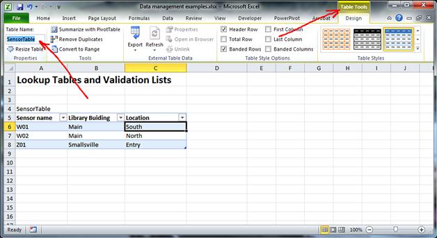
After you have inserted a table, you should change its name to something sensible. The default table name will be Table1, then next one will be Table2, etc. Table1 will not be confusing if you only have a few tables. However, if you had say 15 tables, then how are you going to remember what Table11 refers to? You will not remember, so you will spend an inordinate amount of time cross referencing lists, and going back and forth in your spreadsheet. Don’t to this, it is just plain silly. Renaming your tables is very easy. The only rule is you cannot use some characters, including spaces.
In Excel 2010 you can rename the table by clicking on the table to activate the table tool menu, then changing the name in the table name box (see arrows):
You will notice a few changes after you have converted a range to a table. The table will default to banding format, with alternating blue and white rows. This is just an esthetic thing. The table will have a little dark blue angle (back to front L) at the bottom right row. This is a handle, and you can grab it to manually expand and contract the table. For the most part you will not need to do this, but it can come in handy on rare occasions. Try creating a table now, and practice moving that handle. While you are practicing, try typing a new heading, just to the right of your table. Notice that the table automatically expands to accommodate the new column. Try adding a new bit of data at the end of the table, and hitting enter. Notice that the table automatically expands to accommodate the new row. So tables are dynamic. They will expand as you add new data.
The other dynamic thing about tables is they automatically fill a formula down to the last table row in a column. This means users can add data, and the formulas will be automatically added for those rows. You will also notice that the formula syntax for tables is slightly different. The following is just nonsense data, so as that you can see how the table works without being distracted by real data. I created three headers, “Value 1”, “Value 2”, and “Sum.” After entering four rows of data under “Value 1” and “Value 2” I selected the cells A1 to C5, and inserted a table. Try doing this now yourself. Then click on the cell C2, and type “=” (without the quotation marks of course!), and then click on cell A1, type “+”, then click on cell B2. You will see that the syntax for tables is very different, with the formulas referring to the column headers using “[@[headername]]” format. This is the only thing that is different, all other aspects to crafting formulas remain unchanged. If you build the formula from within the table, by clicking on the cells, Excel will automatically add the field names. You will also notice that when you hit return, the formula will automatically fill down. If you added a value in cell A6, and hit return, you will see the table expands, and the formula is added to C6.

You can delete a row from a table by clicking on a cell, right clicking, and choosing “Delete”>“Table Rows.” The wonderful thing is, if you delete a row in this fashion, Excel only deletes the row in the table. Any rows outside the table will not be affected. The same applies to columns.
Finally, you will see that when you create a table the headers all get an inverted triangle icon placed next to them. If you click on this triangle, a menu will pop up for that column header. You can use the menu to sort the list, you can search for values using a range of Boolean type functions, you can do a quick search using the search box, or you can filter using the check box.
Using a table to populate a validation list
To populate a validation list with the contents from a column in a table, the first thing you need to do is to create the table. Once you have done this, select the column in your raw data table to which you wish to apply the data validation. In this example, I am applying data validation to the sensor name for our Library Visits spreadsheet. This will ensure that users cannot make up a sensor name that does not exist, they have to choose a real sensor from a list that I give them.
I created the below table, and named it “SensorTable”

I then went to my raw data sheet, selected column D, activated the Data Validation dialogue box, selected allow list, then entered the following formula: =INDIRECT(“SensorTable[Sensor Name]”)

How does this formula work? The INDIRECT formula allows you to indirectly refer to a cell, named range, or range. It’s a bit like when you were at school, and you were keen on someone but too scared of being rejected, so you put a friend up to asking that person whether they liked you too. You get the answer, but not directly from the person you are interested in, you get the answer via your friend. The INDIRECT formula does a similar thing. In this example, the size of the SensorTable would change if we added sensors to the table. So we cannot refer to a fixed range, i.e., we cannot hard wire this in directly, as we don’t know how big the SensorTable will be in future. This formula in effect is saying, I don’t know how big the SensorTable is, so please go off and ask the SensorTable how big it is, then I will use that information to determine how many values I will put into the validation list.
If you are still worried about how the formula works, don’t be. All you need to do is plug in the relevant table and header names into the formula.
Dependent lookups
The last type of lookup is a dependent lookup. There might be occasions where you want users to have different values to choose from in the lists, depending upon the information they provided previously. For example, if you are collecting information about the types of help you are providing at various service points, then you would probably want a different list of items staff could help clients with, depending upon the type of help provided by the staff member. A person that provides help at the information desk may answer questions about where to find the toilets, but never be expected to answer questions about where to find information on executives in the car industry.
By far the easiest way to create dynamic dependent lookups is to use tables. Unfortunately, Excel throws a few obstacles in the path of creating dynamic dependent lookups, but there is a work around that is not too complex. Firstly, here is an example in case you do not know what a dependent look up means.

I have committed the sin of putting my raw data on the same sheet as my validation lists, but I only committed this sin so as that you can see the relationship between the dependent lookups and the validation lists more easily. In cell A14 I have selected “Reference Help Desk,” which means the values I can select in cell B14 are “Search interface,” “Database content,” etc. If I changed cell A14 to “Roving staff,” then the values I would be able to select in cell B14 would be different, they would be “IT” and “Finding resources.” Now please put aside any concerns you might have about the terminology I used, or whether the items in the list are mutually exclusive. It’s the concept that counts here, and the concept is that there will be times when you might want to vary the content of a validation list, depending upon the value the user selects in another cell. This is why it is called a dependent lookup, the content of one validation list depends upon the value of another cell.
To create a dynamic dependent lookup you need to do the following:
• Define the content of your primary list, and identify what table each value in the list should point to. In the above, for example, the primary list is defined by cells A5 to B8. This table contains a row for each service, and in column B a list of table and field names for the dependent lookup. For example, cell A6 contains the service “Information Desk,” and the cell to the right contains the value “InfoDeskList[Information Desk].” “InfoDeskList” is the name of the table starting in cell D5, and “[Information Desk]” is the name of the field (i.e., the column header in cell D5). The primary list table (A5:B8) is used to tell Excel where to find the dependent lookup for any value a user selects in column A of that table.
• Create a dynamic named range for the primary list table. This is a workaround that is necessary to overcome a limitation in the formulas that can be used for validation lists. Because I put the raw data in the same sheet as the validation lists (which you should never do), I had to use a modified version of the formula for which you should now be very familiar: =OFFSET(Validation!$A$6,0,0,COUNTA(Validation!$A$6:$A$11),2). I named this range “ServiceDNR,” and named the table occupying cells A5 to B8 “ServiceTable.”
• Next you will need to create a separate table for each dependent lookup. These are the three tables starting in cells D5, F5 and H5 – i.e., the tables with the column headers of “Information Desk,” “Reference Help Desk,” and “Roving Staff,” Name these tables something sensible – i.e., a short but intuitive name that follows a consistent naming format. I have named these tables as lists, rather than tables, to reflect the fact that they only have one column. You don’t need to do this; you just need to be consistent and meaningful in your name format.
• The next step is to add the data validation to your raw data table. There are two data validation lists you need to add; one for the service, and one for the query. In my raw data sheet, which in this example starts on row 12, I pointed the data validation list for the Service column (i.e., rows A14 down) to the first column in my ServiceTable (i.e., the table occupying cells A5 to B8). I have done this by selecting cell A14, opening the data validation dialogue box, selecting allow list, and inserting the following formula:
=INDIRECT(“ServiceTable[Service]”). This formula asks Excel to retrieve the first column from the ServiceTable (i.e., the [Service] field), and put the values in that field into the validation list. After you do this, you will find when you click in cell A14 that you have a choice to enter one of three values, “Information Desk,” “Reference Help Desk,” or “Roving Staff.” If you added a value to A9, then that would also appear in the validation list for service.
• The final step is to add the dependent lookup for the “Query” column in your raw data sheet. Once again, select cell B14, open the data validation dialogue box, select allow list, and insert the following formula:
=INDIRECT(VLOOKUP($A14, ServiceDNR, 2, FALSE))
The VLOOKUP part of the formula gets the value in the cell to the left (e.g., “Reference Help Desk”), then looks for that in the range called “ServiceDNR.” It finds the value “Reference Help Desk” in row A7 of that table. The formula then looks for the value in the second column of “ServiceDNR”, which happens to be “RefDeskList[Reference Help Desk].” The false bit just means make sure it is an exact match. So “VLOOKUP($A14, ServiceDNR, 2, FALSE)” returns the value ‘RefDeskList[Reference Help Desk].” When the VLOOKUP part of the formula is substituted with the value found by VLOOKUP, the formula looks like this =INDIRECT(‘RefDeskList[Reference Help Desk]”). The INDIRECT formula asks Excel to find the values in the table “RefDeskList”, and return all those it finds in that table under the field heading “Reference Help Desk.” So in this example, the validation list for cell B14 becomes “Search interface,” “Database content,” etc.
• To apply the validation list to other cells, simply select a range that includes the cell with the validation, then open the validation dialogue box. Excel will then ask you if you want to extend the validation rules to the other cells, to which you click yes, then OK.
Dynamic dependent lookups are a bit more involved, but once you have done it, you can just set and forget. The only time you will need to fiddle with the formulas is if you add a Service. Once you have written these formulas, you will find them much easier the next time around.
The alternative to using dependent lookups would be to have all the values for each service appear in the validation list. This will become a problem, because it will allow staff to use the data in ways you probably did not intend. For example, as staff member providing roving support might say that they answered a query on research support. If all staff can provide any support, i.e., you have a truly multitasked front line staff, then you will not need dependent lists for this spreadsheet. Otherwise, if you do provide specialized support, then dependent lookups will help to maintain data integrity.