
Chapter 3. Dynamical Quadrature Grids
Applications in Density Functional Calculations
Nathan Luehr, Ivan Ufimtsev and Todd Martinez
In this chapter we present a GPU accelerated quadrature grid scheme designed for situations where the grid points move in time. We discuss the relative merits of several schemes for parallelization, introduce mixed precision as a valuable optimization technique, and discuss problems arising from necessary branching within a warp.
3.1. Introduction
Quadrature grids are often custom built to match the topography of a particular integrand. For example, additional points may be allotted near known discontinuities. A subtle complication arises when the integrand evolves in time. In such cases, the quadrature points dynamically follow features of the integrand. As a result the grid depends on the motion of the system and contributes to its gradient. Standard quadrature schemes are unstable in the present context because they assume the grid is static and do not possess well-behaved gradients.
Kohn-Sham density functional theory (DFT) is one application where these considerations arise
[1]
. DFT replaces the Hamiltonian for interacting electrons in the field of nuclear point charges with a corresponding independent particle Hamiltonian. The independent electrons are then subjected to an additional density-dependent “Kohn-Sham” potential that constrains the noninteracting system to maintain the same charge density as the interacting system it models. Not surprisingly, the form of the Kohn-Sham potential is too complicated for analytical integration, and it must be treated with quadrature grids.
(3.1)
(3.2)
3.2. Core Method
The approach to dynamical grids used in chemical DFT calculations was introduced by Becke
[3]
. A set of independent and overlapping spherical quadratures with weights
 and coordinate offsets
 are centered at each atomic position,
 . The independent quadratures are then harmonized with an additional Becke weight,
 , that allows each atomic-centered quadrature to dominate in the vicinity of its central atom and that forces it to zero in the vicinity of other atoms. In terms of the notation introduced above
 The spherical quadrature weight, for example, from Lebedev's formulas
[4]
, is a constant so that only the Becke weight needs to be a continuous function of the atomic positions. This is effected by defining the Becke weight in terms of the confocal elliptical coordinate,
The spherical quadrature weight, for example, from Lebedev's formulas
[4]
, is a constant so that only the Becke weight needs to be a continuous function of the atomic positions. This is effected by defining the Becke weight in terms of the confocal elliptical coordinate,
 :
:
 where
where
 and
and
 again represent the locations of the
 and
and
 atoms, respectively, and
 is the position of an arbitrary quadrature point.
 is limited to the range
 and measures the pair-wise proximity of r to the
 atom. A polynomial cutoff function,
 , is defined that runs smoothly from
 to
to
 . The following piecewise form has been recommended for
 , along with a value of 0.64 for the parameter
 [5]
, as shown in
Figure 3.1
.
[5]
, as shown in
Figure 3.1
.
(3.3)
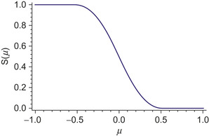 |
| Figure 3.1
Plot of cutoff function,
|
The cutoff function accounts for only a single neighbor atom. To include all of the atoms, a series of cutoff functions are multiplied, each of which accounts for a different neighbor atom. Finally, the cutoff product must be normalized to eliminate double counting from different atomic quadratures.
 A naïve approach would allow the atomic indexes in
Eq. 3.4
to run over all atoms in the system. Since the number of grid points is proportional to the number of atoms, this leads to a formal scaling of
A naïve approach would allow the atomic indexes in
Eq. 3.4
to run over all atoms in the system. Since the number of grid points is proportional to the number of atoms, this leads to a formal scaling of
 for the calculation of all weights. However, because density functional integrands decay exponentially to zero away from the nuclei, a radial cutoff can be introduced in each of the spherical quadratures. As a result, each point needs to consider only the small set of nearby atoms whose spherical quadratures contain it. For large systems, the number of significant neighbors becomes constant leading to linear scaling.
(3.4)
3.3. Implementation
We have implemented the linear-scaling Becke algorithm within a developmental version of the TeraChem quantum chemistry package
[6]
. Our grids are used to calculate the exchange-correlation component of the total energy and Kohn-Sham Fock matrix.
We chose to use the GPU only for the Becke weight portion of quadrature generation because this step dominates the runtime of the grid setup procedure. Before the kernel is called, the spherical grids are expanded around each atom by table lookup, the points are sorted into spatial bins, and neighbor lists are generated for each bin. These steps are nearly identical for our CPU and GPU implementations. The table lookup and point sorting are already very fast on the CPU, and no GPU implementation is planned. Building atom lists for each bin is more time-consuming and may benefit from further GPU acceleration in the future, but it is not a focus of this chapter.
The GPU is used to calculate the Becke weights given by
Eq. 3.4
. Since the denominator includes the numerator as one of its terms, we focus on calculating the former, setting aside the numerator in a variable when we come upon it. The serial implementation falls naturally into the triple loop pseudo-code listing in
Figure 3.2
.
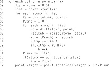 |
| Figure 3.2
Pseudo-code listing of Becke kernel as a serial triple loop.
|
In order to accelerate this algorithm on the GPU, we first needed to locate a fine-grained yet independent task to serve as the basis for our device threads. These arise naturally by dividing loop iterations in the serial implementation into CUDA blocks and threads. Our attempts at optimization fell into two categories. The finest level of parallelism was to have each block cooperate to produce the weight for a single point (block per point). In this scheme CUDA threads were arranged into 2-D blocks. The y-dimension specified the atomA index, and the x-dimension specified the atomB index (following notation from
Figure 3.2
). The second optimization scheme split the outermost loop and assigned an independent thread to each weight (thread per point).
In addition to greater parallelism, the block-per-point arrangement offered an additional caching advantage. Rather than recalculating each atom-to-point distance (needed at lines 5 and 8), these values were cached in shared memory, avoiding roughly nine floating-point operations in the inner loop.
Unfortunately, this boost was more than offset by the cost of significant block-level cooperation. First, lines 11 and 14 required block-level reductions in the x and y dimensions, respectively. Second, because the number of members in each atom list varies from as few as 2 to more than 80 atoms, any chosen block dimension was necessarily suboptimal for many bins. Finally, the early exit condition at line 12 proved problematic. Since
 falls between 0.0 and 1.0, each iteration of the atomB loop can only reduce the value of P_tmp. Once it has been effectively reduced to zero, we can safely exit the loop. As a result, calculating multiple “iterations” of the loop in parallel required wasted terms to be calculated before the early exit was reached.
The thread-per-point approach did not suffer from its coarser parallelism. In the optimized kernel each thread required a modest 29 registers and no shared memory. Thus, reasonable occupancies of 16
warps per streaming multiprocessor (SM) were obtained (using a Tesla C1060 GPU). Since a usual calculation requires millions of quadrature points (and thus threads), there was also plenty of work available to saturate the GPU's resources.
The thread-per-point implementation was highly sensitive to branching within a warp. Because each warp is executed in SIMD fashion, neighboring threads can drag each other through nonessential instructions. In the thread-per-point implementation, this can happen in two ways: (1) a warp contains points from bins with varying neighbor list lengths or (2) threads in a warp exit at different iterations of the inner loop. Since many bins have only a few points and thus warps often span multiple bins, case one can become an important factor. Fortunately, it is easily mitigated by presorting the bins such that neighboring warps will have similar loop limits.
The second case was more problematic and limited initial versions of the kernel to only 132 GFLOPS. This was only a third of the Tesla C1060's single issue potential. Removing the early exit and forcing the threads to complete all inner loop iterations significantly improved the GPU's floating-point throughput to 260 GFLOPS, 84% of the theoretical peak. However, the computation time also increased, as the total amount of work more than tripled for our test geometry.
To minimize branching, we need to further sort the points within each bin such that nearest neighbors were executed in nearby threads. In this way, each thread in a warp behaved as similarly as possible under the branch conditions in the code. This adjustment provided a modest performance increase to 149 GFLOPS. Further tweaking ultimately allowed 187 GFLOPS of sustained performance, about 60% of the single-issue peak. However, thread divergence remains a significant barrier to greater efficiency. These results demonstrate the sensitivity of CUDA hardware to even simple branching conditions.
After the bins and points have been sorted on the host, the data is moved to the GPU. We copy each point's Cartesian coordinates, spherical weights ( in
Eq. 3.3
), central atom index, and bin index to GPU global memory arrays. The atomic coordinates for each bin list are copied to the GPU in bin-major order. This order allows threads across a bin barrier to better coalesce their reads — a step that is necessary since threads working on different bins often share a warp.
in
Eq. 3.3
), central atom index, and bin index to GPU global memory arrays. The atomic coordinates for each bin list are copied to the GPU in bin-major order. This order allows threads across a bin barrier to better coalesce their reads — a step that is necessary since threads working on different bins often share a warp.
Once the data is arranged on the GPU, the kernel is launched, calculates the Becke weight, and combines it with the spherical weight in place. Finally, the weights are copied back to the host and stored for later use in the DFT calculation.
Because the GPU is up to an order of magnitude faster using single- rather than double-precision arithmetic, our kernel was designed to minimize double-precision operations. Double precision is most important when accumulating small numbers into larger ones or when taking differences of nearly equal numbers. With this in mind we were able to improve our single-precision results using only a handful of double-precision operations. Specifically, the accumulation at line 14 and the final arithmetic of line 17 were carried out in double-precision. This had essentially no impact on performance, but improved correlation with the full double-precision results by more than an order of magnitude, as shown in
Table 3.1
.
3.4. Performance Improvement
We compared our production mixed precision GPU code with a CPU implementation of the same algorithm. To level the playing field, we had the CPU code use the same mixed precision scheme developed for the GPU. However, the CPU implementation's serial structure limited its computation to a single core. The reference timings were taken using an Intel Xeon X5570 at 2.93 GHz and an
NVIDIA Tesla C1060 GPU. Quadrature grids were generated for a representative set of test geometries ranging from about 100 to nearly 900 atoms.
Table 3.2
compares the CPU and GPU Becke kernel implementations (code corresponding to
Figure 3.2
) for the test molecules shown in
Figure 3.3
. The observed scaling is not strictly linear with system size. This is because the test molecules exhibit varying atomic densities. When the atoms are more densely packed, more neighbors appear in the inner loops. We can use the average size of the neighbor lists for each system to crudely account for the variation in atomic density. Doing so produces the expected linear result, as shown in
Figure 3.4
.
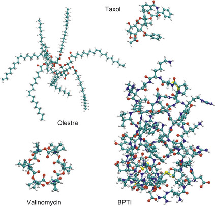 |
| Figure 3.3
Test molecules.
|
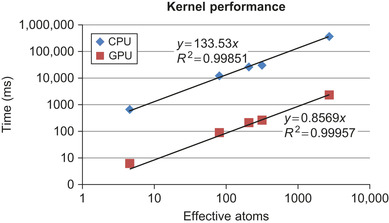 |
| Figure 3.4
Plot showing linear scaling of CPU and GPU kernels. Slope of linear fit gives performance in terms of ms per effective atom.
|
Although a speedup of up to 150X over a state-of-the-art CPU is impressive, it ignores the larger picture of grid generation as a whole. In any real-world application the entire procedure from spherical grid lookup to bin sorting and memory transfers must be taken into account.
Table 3.3
provides a timings breakdown for the BPTI test geometry.
The massive kernel improvement translates into a 38X global speedup. Clearly, we have been successful in eliminating the principal bottleneck in the CPU code. The Becke kernel accounts for up to 98% of the total CPU runtime, but on the GPU it is overshadowed by the previously insignificant atom list step. This is a practical example of Amdahl's law, which states that the total speedup is limited by the proportion of code that is left unparallelized.
3.5. Future Work
From the preceding discussion, the obvious next step will be to implement a GPU accelerated nearest neighbor algorithm to build the atom lists in place on the GPU. Although neighbor listing is not ideally
suited for GPU acceleration, use of new features available on NVIDIA's Fermi architecture, such as faster atomics and more robust thread synchronization, should allow a modest speedup. And any gain at this step will amplify the kernel speedup attained thus far.
A second direction for further work is the implementation of GPU accelerated weight gradients (needed in
Eq. 3.2
). Preliminary tests show that these too are excellent candidates for GPU acceleration.
References
[1]
A good overview of DFT can be found in
K. Yasuda,
Accelerating density functional calculations with graphics processing unit
,
J. Chem. Theory Comput.
4
(2008
)
1230
–
1236
;
For detailed coverage see R.G. Parr, W. Yang, Density Functional Theory of Atoms and Molecules, Oxford University Press, New York, 1994
.
[2]
B.G. Johnson, P.M.W. Gill, J.A. Pople,
The performance of a family of density functional methods
,
J. Chem Phys.
98
(1993
)
5612
.
[3]
A.D. Becke,
A multicenter numerical integration scheme for polyatomic molecules
,
J. Chem. Phys.
88
(1988
)
2547
.
[4]
V.I. Lebedev, D.N. Laikov,
A quadrature formula for the sphere of the 131st algebraic order of accuracy
,
Dokl. Math.
59
(1999
)
477
–
481
.
[5]
R.E. Stratmann, G.E. Scuseria, M.J. Frisch,
Achieving linear scaling in exchange-correlation density functional quadratures
,
Chem. Phys. Lett.
257
(1996
)
213
–
223
.
[6]
I.S. Ufimtsev, T.J. Martinez,
Quantum chemistry on graphical processing units. 3. Analytical energy gradients, geometry optimization, and first principles of molecular dynamics
,
J. Chem. Theory Comput.
5
(2009
)
2619
–
2628
.
..................Content has been hidden....................
You can't read the all page of ebook, please click here login for view all page.