
Chapter 7. Leveraging the Untapped Computation Power of GPUs
Fast Spectral Synthesis Using Texture Interpolation
Richard Townsend, Karthikeyan Sankaralingam and Matthew D. Sinclair
In this chapter we develop a hardware/software platform,
grassy
, that takes a unique approach to computation on GPUs by leveraging the interpolation capability of GPU texture memory. Our solution is motivated by the computational needs of asteroseismology, which we briefly outline. Beyond the specific application to asteroseismology, our work provides the first investigation into the use of texture interpolation functionality for non-graphics computations.
7.1. Background and Problem Statement
7.1.1. Asteroseismology
Asteroseismology
is a powerful technique for probing the internal structure of distant stars by studying time-varying disturbances on their surfaces. A direct analogy can be drawn to the way that the study of earthquakes (seismology) allows us to infer the internal structure of the Earth. Due to the recent launch of space satellites devoted to discovering and monitoring these surface disturbances in hundreds of thousands of stars, paired with ground-based telescopes capable of high-resolution, high-cadence follow-up spectroscopy, asteroseismology is currently enjoying a golden age. However, there remains a significant computation challenge: how do we analyze and interpret the veritable torrent of new asteroseismic data?
To date, the most straightforward and accurate analysis approach is direct modeling via spectral synthesis (discussed in greater detail later in this chapter). Given a set of observations of the time-varying radiant flux received from a star, we attempt to construct a sequence of synthetic spectra to reproduce these observations. Any given model depends on the assumed parameters describing the star and its surface disturbances. Using an optimization strategy we find the combination of parameters that best reproduces the observations, ultimately allowing us to establish constraints on the stellar structure.
Stellar spectral synthesis is the process of summing up the Earth-directed radiant flux from each region on the visible hemisphere of a star. A typical procedure, e.g., Reference 1, comprises the following steps:
1.
Mesh building
. Decompose the stellar surface into a triangle mesh (Figure 7.1a
). A quad [
T
,
g
,
v
,
μ
] (see
Table 7.1
) is associated with each mesh vertex (Figure 7.1b
).
2.
Mesh rendering
. Rasterize the view-plane projection of every triangle to produce a set of
N
frag
equal-area fragments (Figure 7.1c
). Bilinear interpolation between triangle vertices is used to calculate a quad [
T
,
g
,
v
,
μ
] for each fragment.
3.
Flux calculation
. Evaluate the radiant flux spectrum
F
(λ
j
) on a uniformly spaced grid of
N
λ
discrete wavelengths
λ
j
=
λ
0
+ Δ
λ
j
(j
= 0…
N
λ
− 1) for each fragment (Figure 7.1d
).
4.
Flux aggregation
. Sum the
N
frag
flux spectra to produce a single synthetic spectrum representing the radiant flux for the whole star (Figure 7.1e
).
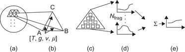 |
| Figure 7.1
Steps in the spectral synthesis procedure (see
Section 7.1.2
).
|
Steps (1) and (2) are performed once for a star and/or set of stellar and disturbance parameters. The main computational cost comes in step (3), which we now discuss in greater detail.
Over the wavelength grid
λ
j
the radiant flux is calculated as
 Here,
A
is the area of the fragment,
D
the distance to the star, and
I
(…) the specific intensity of the radiation emerging at rest wavelength
Here,
A
is the area of the fragment,
D
the distance to the star, and
I
(…) the specific intensity of the radiation emerging at rest wavelength
 and direction cosine
μ
from a stellar atmosphere with effective temperature
T
and surface gravity
g
(see
Table 7.1
). The rest wavelength is obtained from the Doppler shift formula,
and direction cosine
μ
from a stellar atmosphere with effective temperature
T
and surface gravity
g
(see
Table 7.1
). The rest wavelength is obtained from the Doppler shift formula,
 where
v
is the line-of-sight velocity of the fragment and
c
is the speed of light.
where
v
is the line-of-sight velocity of the fragment and
c
is the speed of light.
(7.1)
(7.2)
7.1.3. Problem Statement
For typical parameters (N
frag
,
N
λ
≈ 5,000−10,000) a synthetic spectrum typically takes only a few seconds to generate on a modern CPU. However, with many possible parameter combinations, the overall optimization (see
Section 7.1.1
) can be computationally expensive, taking many weeks in a typical analysis. The primary bottleneck lies in the 4-D specific intensity interpolations described earlier in this chapter; although algorithmically simple, their arithmetic and memory-access costs quickly add up. This issue motivates us to pose the following question:
How can we use GPUs to accelerate interpolations in the precomputed specific intensity tables?
In addressing this question, we have developed
grassy
(GR
aphics Processing Unit —
A
ccelerated
S
pectral
SY
nthesis) — a hardware/software platform for fast spectral synthesis that leverages the texture interpolation functionality in CUDA-capable GPUs (see
Figure 7.2
). In the following section, we establish a more formal basis for the interpolation problem; then, in
Section 7.3
, we introduce our
grassy
platform.
Section 7.4
presents results from initial validation and testing, and in
Section 7.5
, we discuss future directions for this avenue of GPU computing research.
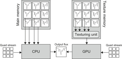 |
| Figure 7.2
Schematic comparison of CPU and GPU spectral synthesis.
|
7.2. Flux Calculation and Aggregation
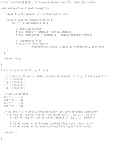
An example of CPU-oriented pseudo code for the flux calculation and aggregation steps (3 and 4) of the spectral synthesis procedure (Section 7.1.2
) is given in
Listing 7.1
. Input to the code is a stream of quads from the mesh building and rasterization steps (1 and 2); the output is the aggregated synthetic spectrum. The high arithmetic and memory-access costs of the 4-D specific intensity interpolation are evident in the 16-term weighted summation appearing toward the end of the code — this expression must be evaluated
N
frag
N
λ
times during the synthesis of a single spectrum.
7.3.1. Overview
In this section, we introduce the
grassy
spectral synthesis platform. To leverage the texture interpolation functionality in CUDA-capable GPUs, some modifications to the procedure outlined in
Listing 7.1
are necessary. In particular, we decompose the calculations into a series of 2-D interpolations, which are then implemented as fetches (with bilinear filtering) from 2-D textures. This brings the dual benefits of efficient memory access due to use of the texture cache, and “free” interpolation arithmetic provided by the linear filtering mode. One potential pitfall, however, is the limited precision of the linear filtering; we review this issue in
Section 7.3.6
.
7.3.2. Interpolation Decomposition
The 4-D to 2-D interpolation decomposition is enabled by a CPU-based preprocessing step, whereby quads [
T
,
g
,
v
,
m
] from step (2) of the spectral synthesis procedure are translated into 10-tuples [
v
,
μ
,
k
0
,
k
1
,
k
2
,
k
3
,
w
0
,
w
1
,
w
2
,
w
3
]. A single 10-tuple codes for four separate bilinear interpolations, in 2-D tables
 representing the specific intensity for a given combination of effective temperature and surface gravity. The indices
 indicate
which
tables to interpolate within, while the weights
w
0
…
w
3
are used post-interpolation to combine the results together.
indicate
which
tables to interpolate within, while the weights
w
0
…
w
3
are used post-interpolation to combine the results together.
7.3.3. Texture Packing
Because CUDA does not support arrays of texture references (which would allow us to place each table into a separate texture),
grassy
packs the 2-D intensity tables
 into a single 2-D texture.
1
For a given interpolation, the floating-point texture coordinates (x
,
y
) are calculated from
λ
,
μ
and the table index
k
via
into a single 2-D texture.
1
For a given interpolation, the floating-point texture coordinates (x
,
y
) are calculated from
λ
,
μ
and the table index
k
via
 and
and
 Here,
Here,
 is the direction cosine dimension of each intensity table, while
 is the base wavelength and
 the wavelength spacing (not to be confused with
λ
and Δ
λ
). The offsets by 0.5 come from the recommendations of Appendix F.3 of
[10]
. Note that these two equations are
not
the actual interpolation, but rather the conversion from physical (wavelength, direction cosine) coordinates to un-normalized texture coordinates.
the wavelength spacing (not to be confused with
λ
and Δ
λ
). The offsets by 0.5 come from the recommendations of Appendix F.3 of
[10]
. Note that these two equations are
not
the actual interpolation, but rather the conversion from physical (wavelength, direction cosine) coordinates to un-normalized texture coordinates.
(7.3)
(7.4)
7.3.4. Division of Labor
To maximize texture cache locality,
grassy
groups calculations into
N
b
batches of
 consecutive wavelengths. These batches map directly into CUDA thread blocks, with each thread in a block
responsible for interpolating the intensity, and accumulating the flux, at a single wavelength. To ensure adequate utilization of GPU resources,
N
b
should be an integer multiple of the number of streaming multiprocessors (SMs) in the device.
consecutive wavelengths. These batches map directly into CUDA thread blocks, with each thread in a block
responsible for interpolating the intensity, and accumulating the flux, at a single wavelength. To ensure adequate utilization of GPU resources,
N
b
should be an integer multiple of the number of streaming multiprocessors (SMs) in the device.
Every thread block processes the entire input stream of
N
frag
10-tuples, to build up the aggregated flux spectrum for the wavelength range covered by the block. Upon completion, this spectrum is written to global memory, from where it can subsequently be copied over to the CPU.
7.3.5. Pseudo Code
Listing 7.2
provides pseudo code for the CUDA kernel within
grassy
, which handles the flux calculation and aggregation. Kernel arguments are the input stream of 10-tuples and a pointer to an array in device global memory where the resulting flux spectrum will be placed. Each thread evaluates its own wavelength on the fly from the index
j
, which in turn is obtained from thread and block indices.
7.3.6. Analysis of Precision Issues
In this subsection we discuss in detail the potential issues arising from the 9-bit precision of the GPU texture interpolation. For exact one-dimensional linear interpolation between two pairs of points, (x
0
,
f
0
) and (x
1
,
f
1
), the interpolant
f
(x
) can be expressed as
 Here,
Here,
 is the weight function, whose linear variation between 0 (x
=
x
0
) and 1 (x
=
x
1
) gives a corresponding linear change in
f
(x
), from
f
=
f
0
to
f
=
f
1
. In a floating-point implementation of these expressions, the finite precision means that
f
(x
) no longer varies completely smoothly, instead exhibiting step-wise jumps. However, these jumps are typically on the order of a few units of last place and thus not a particularly important source of numerical error.
is the weight function, whose linear variation between 0 (x
=
x
0
) and 1 (x
=
x
1
) gives a corresponding linear change in
f
(x
), from
f
=
f
0
to
f
=
f
1
. In a floating-point implementation of these expressions, the finite precision means that
f
(x
) no longer varies completely smoothly, instead exhibiting step-wise jumps. However, these jumps are typically on the order of a few units of last place and thus not a particularly important source of numerical error.
(7.5)
(7.6)
The situation is different if the weight function
w
(x
) is evaluated using fixed-precision arithmetic. With
n
bits of precision, there are only 2
n
distinct values that
w
(x
) can assume — and, by implication, only 2
n
distinct values of
f
(x
) between
f
0
and
f
1
. Then, the step-wise jumps in
f
(x
) can be significant.
Exactly how significant the step-wise jump is depends on the difference between
f
0
and
f
1
. The worst-case scenario occurs when
f
1
= −
f
0
, giving a bound on the error in
f
(x
) of
 For the fixed-precision linear interpolation offered through CUDA texture lookups,
n
= 9 bits, giving an error bound of
For the fixed-precision linear interpolation offered through CUDA texture lookups,
n
= 9 bits, giving an error bound of
 . However, in practice the error will be much smaller than this because for an adequately sampled lookup table the worst-case scenario will never arise. If all features in the table have a characteristic width of
m
points, then the maximum difference between
f
0
and
f
1
is
f
/
m
, giving an error bound
. However, in practice the error will be much smaller than this because for an adequately sampled lookup table the worst-case scenario will never arise. If all features in the table have a characteristic width of
m
points, then the maximum difference between
f
0
and
f
1
is
f
/
m
, giving an error bound

Clearly, a more-finely sampled table (i.e., larger m
) yields smaller errors, at the cost of consuming more memory.
(7.7)
(7.8)
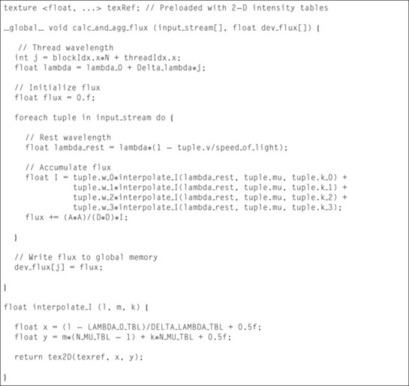 |
| Listing 7.2. |
| Pseudo code for the grassy kernel.
|
In the present context of specific intensity interpolation, we use tables sampled at 0.03 Angstrom. Over the optical wavelength range of 3,500–7,500 Angstrom, features in the tables have a typical scale of at least 0.2 Angstrom (the thermal broadening width), six times the sampling interval. This implies an error bound (assuming
n
= 9) of
 . Errors of this magnitude are unimportant when contrasted against uncertainties in the tabulated intensities (due to theoretical approximations) and against the inherent noise in the observations against which synthetic spectra are compared.
In anticipation of the performance evaluation in the following section, here we provide a simple model to estimate the expected performance of
grassy
. Let
 be the number of computational operations required to process one 10-tuple at one wavelength; the total number of operations for synthesis of a complete spectrum is then
 . For
. For
 (typical values, and the ones adopted in the calculations below), and assuming
 , we estimate
 billion operations (GOPS) per spectrum.
A Tesla C1060 GPU has a peak throughput of 933 GOPS/s. Assuming we are able to achieve half of this, we expect a throughput of 70 spectra per second, or 14 ms per spectrum.
7.4. Initial Testing
7.4.1. Platform and Infrastructure
Our testing and validation platform is a Dell Precision 490 workstation, containing two 2.33 GHz Intel Xeon E5345 quad-core CPUs and a Tesla C1060 GPU. The workstation runs 64-bit Gentoo Linux (kernel 2.6.25) and uses version 3.0 of the CUDA SDK. As a CPU-based comparison code, we adopt a highly optimized Fortran 95 version of the
kylie
code
[1]
, running on the same workstation.
7.4.2. Performance Evaluation
Table 7.2
summarizes the average time taken by the CPU and GPU platforms to synthesize a spectrum with
 . For these calculations, we adopt a GPU thread block size of 128; a gradual performance degradation occurs toward larger values of the block size because of a shortage of blocks to map on to multiprocessors.
| Platform | Time (ms) |
|---|---|
| CPU/Xeon E5345 | 1490 |
| GPU/Tesla C1060 | 55.1 |
As mentioned in
Section 7.1
, the CPU platform takes on the order of seconds per spectrum. The Tesla C1060 is around 30 times faster than the CPU, although not so fast as we had estimated from our simple analysis in
Section 7.3.7
. The bottleneck appears to be in the memory accesses; the global memory throughput reported by the
cudaprof
profiler is only 17.1 GB/sec. On closer inspection, it appears that we are not making best use of the texture cache; the ratio of misses to hits is an alarming 90:1! We are currently examining ways in which better cache locality might be achieved, for instance, by altering the texture-packing layout (Section 7.3.3
).
7.5.1. Asteroseismology
As we have discussed already in this chapter, specific intensity interpolation currently represents the major bottleneck in synthesizing spectra for asteroseismic analyses. Current CPU-based implementations typically lead to per-star analysis runtimes of weeks. The speedups reported earlier in this chapter — when scaled to multidevice systems — herald the prospect of being able to shorten these times to hours. It goes without saying that this will have a significant impact on the field of asteroseismology, as the analysis throughput and/or resolution of parameter determinations can be greatly increased, in turn allowing stronger constraints to be placed on the internal structures of stars.
7.5.2. Other Areas of Astrophysics
The benefits of accelerated spectral synthesis will also extend to other fields of astrophysics, from the analysis of rotationally flattened stars to the generation of combined spectra for clusters or entire galaxies of stars (so-called population synthesis). Our approach generalizes to other numerical techniques that rely on interpolation as well.
7.5.3. Numerical Analysis
In terms of numerical analysis, our work opens up new avenues. While building this application and investigating the use of textures for computation, we realized several features from a numerical standpoint that introduce trade-offs:
• Sampling: If the data used to populate the interpolation tables are sampled too coarsely, there is loss of precision. However, if sampled too finely the total size of the textures increases.
• Conservative interpolation: Our intensity interpolation scheme is not strictly conservative, in that the integral of the interpolated intensity over a finite wavelength interval will differ somewhat from the corresponding integral of the tabulated intensity. This issue can be resolved by interpolating instead in the cumulative intensity and then taking finite differences. However, such an approach will involve calculating the difference between two large similar numbers, running the risk of catastrophic cancellation. Further research is therefore required to examine how this approach can be implemented safely.
7.5.4. Code Status
Our initial prototype implementation of the code is complete, but optimizations are ongoing. We expect to provide a hosted multiple-device system with remote access for astronomers in the next 12 to 18 months. At this juncture, all source code will be released under the GNU General Public License.
Acknowledgments
We acknowledge support from NSF
Advanced Technology and Instrumentation
grant AST-0904607. The Tesla C1060 GPU used in this study was donated by NVIDIA through its Professor Partnership Program.
The most relevant work in terms of asteroseismology is the
bruce
/
kylie
suite of modeling codes
[1]
. One example of typical analysis using the
bruce
/
kylie
codes is presented in
[2]
. Other works in astronomy that have used GPUs include
[3]
and
[4]
. To the best of our knowledge, the present work is the first use of texture units for computation. In terms of experimental data that
grassy
will analyze, current asteroseismic satellite missions include
[5]
[6]
and
[7]
. The sources for spectral intensity data we use are
[8]
and
[9]
.
[1]
R.H.D. Townsend,
Spectroscopic modelling of non-radial pulsation in rotating early-type stars
,
Mon. Not. R. Astron. Soc.
284
(4
) (1997
)
839
.
[2]
Th. Rivinius, D. Baade, S. Štefl, R.H.D. Townsend, O. Stahl, B. Wolf,
et al.
,
Stellar and circumstellar activity of the Be star mu Centauri. III, Multiline nonradial pulsation modeling
,
Astron. Astrophys. A
369
(2001
)
1058
.
[3]
S.F. Portegies Zwart, R.G. Belleman, P.M. Geldof,
High-performance direct gravitational N-body simulations on graphics processing units
,
New Astron.
12
(8
) (2007
)
641
.
[4]
T. Hamada, T. Iitaka, The chamomile scheme: an optimized algorithm for n-body simulations on programmable graphics processing units. arXiv.org, Cornell University Library, arXiv:astro-ph 0703100. (accessed 10.11.2010).
[5]
J. Christensen-Dalsgaard, T. Arentoft, T.M. Brown, R.L. Gilliland, H. Kjeldsen, W.J. Borucki,
et al.
,
Asteroseismology with the Kepler mission
,
Comm. Astero.
150
(2007
)
350
.
[6]
I. Roxburgh, C. Catala,
The PLATO consortium
,
Comm. Astero.
150
(2007
)
357
.
[7]
G. Handler,
Beta Cephei and Slowly Pulsating B stars as targets for BRITE-Constellation
,
Comm. Astero.
152
(2008
)
160
.
[8]
T. Lanz, I. Hubeny,
Grid of NLTE line-blanketed model atmospheres of early B-type stars
,
Astrophys. J. Suppl. Ser.
169
(1
) (2007
)
83
.
[9]
T. Lanz, I. Hubeny,
A grid of Non-LTE line-blanketed model atmospheres of O-type stars
,
Astrophys. J. Suppl. Ser.
146
(2
) (2003
)
417
.
[10]
NVIDIA CUDA Programming Guide, version 3.0, (accessed 2.20.10).
..................Content has been hidden....................
You can't read the all page of ebook, please click here login for view all page.