
Chapter 9. Treecode and Fast Multipole Method for
N
-Body Simulation with CUDA
Rio Yokota and Lorena A. Barba
The classic
N
-body problem refers to determining the motion of
N
particles that interact via a long-distance force, such as gravitation or electrostatics. A straightforward approach to obtaining the forces affecting each particle is the evaluation of all pair-wise interactions, resulting in
 computational complexity. This method is only reasonable for moderate-size systems or to compute near-field interactions, in combination with a far-field approximation. In the previous
GPU Gems
volume
[21]
, the acceleration of the all-pairs computation on
gpu
s was presented for the case of the gravitational potential of
N
masses. The natural parallelism available in the all-pairs kernel allowed excellent performance on the
gpu
architecture, and the direct kernel of Reference
[24]
achieved over 200 Gigaflops on the
g
e
f
orce
8800 gtx
, calculating more than 19 billion interactions per second with
computational complexity. This method is only reasonable for moderate-size systems or to compute near-field interactions, in combination with a far-field approximation. In the previous
GPU Gems
volume
[21]
, the acceleration of the all-pairs computation on
gpu
s was presented for the case of the gravitational potential of
N
masses. The natural parallelism available in the all-pairs kernel allowed excellent performance on the
gpu
architecture, and the direct kernel of Reference
[24]
achieved over 200 Gigaflops on the
g
e
f
orce
8800 gtx
, calculating more than 19 billion interactions per second with
 . In the present contribution, we have addressed the more involved task of implementing the fast
N
-body algorithms that are used for providing a far-field approximation: the
. In the present contribution, we have addressed the more involved task of implementing the fast
N
-body algorithms that are used for providing a far-field approximation: the
 treecode
[3]
and
treecode
[3]
and
 fast multipole method
[13]
.
fast multipole method
[13]
.
Fast algorithms for
N
-body problems have diverse practical applications. We have mentioned astrophysics, the paradigm problem. Of great importance is also the calculation of electrostatic (Coulomb) interactions of many charged ions in biological molecules. Proteins and their interactions with other molecules constitute a great challenge for computation, and fast algorithms can enable studies at physiologically relevant scales
[4]
and
[26]
. Both gravitational and electrostatic problems are mathematically equivalent to solving a Poisson equation for the scalar potential. A general method for the solution of Poisson problems in integral form is described by Greengard and Lee
[12]
, using the
fmm
in a very interesting way to patch local solutions. In Ethridge and Greengard's work
[9]
, instead, the
fmm
is applied directly to the volume integral representation of the Poisson problem. These general Poisson solvers based on
fmm
open the door to using the algorithm in various situations where complex geometries are involved, such as fluid dynamics, and also shape representation and recognition
[11]
.
The
fmm
for the solution of Helmholtz equations was first developed in Rokhlin's work
[25]
and is explained in great detail in the book by Gumerov and Duraiswami
[14]
. The integral-equation formulation is an essential tool in this context, reducing the volumetric problem into one of an integral over a surface. The
fmm
allows fast solution of these problems by accelerating the computation of dense matrix-vector products arising from the discretization of the integral problem. In fact, the capability
of boundary element methods (bem
) is in this way significantly enhanced; see
[22]
and
[19]
. These developments make possible the use of the
fmm
for many physical and engineering problems, such as seismic, magnetic, and acoustic scattering
[6]
[8]
[10]
and
[16]
. The recent book by Liu
[20]
covers applications in elastostatics, Stokes flow, and acoustics; some notable applications, including acoustic fields of building and sound barrier combinations, and also a wind turbine model, were presented by Bapart, Shen, and Liu
[2]
.
Because of the variety and importance of applications of treecodes and
fmm
, the combination of algorithmic acceleration with hardware acceleration can have tremendous impact. Alas, programming these algorithms efficiently is no piece of cake. In this contribution, we aim to present
gpu
kernels for treecode and
fmm
in, as much as possible, an uncomplicated, accessible way. The interested reader should consult some of the copious literature on the subject for a deeper understanding of the algorithms themselves. Here, we will offer the briefest of summaries. We will focus our attention on achieving a
gpu
implementation that is efficient in its utilization of the architecture, but without applying the most advanced techniques known in the field (which would complicate the presentation). These advanced techniques that we deliberately did not discuss in the present contribution are briefly summarized in
Section 9.6
, for completeness. Our target audience is the researcher involved in computational science with an interest in using fast algorithms for any of the aforementioned applications: astrophysics, molecular dynamics, particle simulation with non-negligible far fields, acoustics, electromagnetics, and boundary integral formulations.
9.2. Fast
N
-Body Simulation
As in Nyland
et al.
[24]
, we will use as our model problem the calculation of the gravitational potential of
N
masses. We have the following expressions for the potential and force, respectively, on a body
 :
:
(9.1)
Here,
 and
and
 are the masses of bodies
 and
and
 , respectively; and
 is the vector from body
 to body
 . Because the distance vector
 is a function of both
 and
and
 , an all-pairs summation must be performed. This results in
 computational complexity. In the treecode, the sum for the potential is factored into a near-field and a far-field expansion, in the following way,
(9.2)
Calculating the summation for
 in this manner can be interpreted as the clustering of particles in the far field. In
Eq. 9.2
,
in this manner can be interpreted as the clustering of particles in the far field. In
Eq. 9.2
,
 is the spherical harmonic function, and
 ;
;
 are the distance vectors from the center of the expansion to bodies
 and
and
 , respectively. The key is to factor the all-pairs interaction into a part that involves only
 and a part that involves only
 , hence allowing the summation of
 to be performed outside of the loop for
 . The condition
 , which is required for the series
expansion to converge, prohibits the clustering of particles in the near field. Therefore, a tree structure is used to form a hierarchical list of
, which is required for the series
expansion to converge, prohibits the clustering of particles in the near field. Therefore, a tree structure is used to form a hierarchical list of
 cells that interact with
N
particles. This results in
cells that interact with
N
particles. This results in
 computational complexity.
The complexity can be further reduced by considering cluster-to-cluster interactions.
1
In the
fmm
, a second series expansion is used for such interactions:
 where the near-field expansion and far-field expansion are reversed. The condition for this expansion to converge is
 , which means that the clustering of particles using
 is only valid in the near field. The key here is to translate multipole expansion coefficients
 of cells in the far field to local expansion coefficients
 of cells in the near field, resulting in a cell-cell interaction. Because of the hierarchical nature of the tree structure, each cell needs to consider only the interaction with a constant number of neighboring cells. Because the number of cells is of
 , the
fmm
has a complexity of
, the
fmm
has a complexity of
 . Also, it is easy to see that keeping the number of cells proportional to
N
results in an asymptotically constant number of particles per cell. This prevents the direct calculation of the near field from adversely affecting the asymptotic behavior of the algorithm.
. Also, it is easy to see that keeping the number of cells proportional to
N
results in an asymptotically constant number of particles per cell. This prevents the direct calculation of the near field from adversely affecting the asymptotic behavior of the algorithm.
(9.3)
1
The groups or clusters of bodies reside in a subdivision of space for which various authors use the term “box” or “cell”; e.g., “leaf-cell” as used in
[24]
corresponds to the smallest subdomain.
The flow of the treecode/
fmm
calculation is illustrated in
Figure 9.1
. This schematic shows how the information of all source particles is propagated to a particular set of target particles. The purpose of this figure is to introduce the naming conventions we use for the seven distinct operations (p2p
,
p2m
,
m2m
,
m2p
,
m2l
,
l2l
,
l2p
), and to associate these steps to a graphical representation. These naming conventions and graphical representations are used later to describe the
gpu
implementation and to assess its performance. The difference between the treecode and
fmm
can be explained concisely using this illustration.
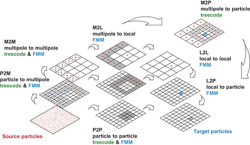 |
| Figure 9.1
Flow of the treecode and
fmm
calculation.
|
First, the mass/charges of the particles are aggregated into the multipole expansions by calculating
 at the center of all cells (the
p2m
operation). Next, the multipole expansions are further clustered by translating the center of each expansion to a larger cell and adding their contributions at that level (m2m
operation). Once the multipole expansions at all levels of the tree are obtained, the treecode calculates
Eq. 9.2
to influence the target particles directly (the
m2p
operation). In contrast, the
fmm
first transforms the multipole expansions to local expansions (m2l
operation) and then translates the center of each expansion to smaller cells (l2l
operation). Finally, the influence of the far field is transmitted from the local expansions to the target particles by calculating
Eq. 9.3
in the
l2p
operation. The influence of the near field is calculated by an all-pairs interaction of neighboring particles (p2p
). In the present contribution, all of the aforementioned operations are implemented as
gpu
kernels.
at the center of all cells (the
p2m
operation). Next, the multipole expansions are further clustered by translating the center of each expansion to a larger cell and adding their contributions at that level (m2m
operation). Once the multipole expansions at all levels of the tree are obtained, the treecode calculates
Eq. 9.2
to influence the target particles directly (the
m2p
operation). In contrast, the
fmm
first transforms the multipole expansions to local expansions (m2l
operation) and then translates the center of each expansion to smaller cells (l2l
operation). Finally, the influence of the far field is transmitted from the local expansions to the target particles by calculating
Eq. 9.3
in the
l2p
operation. The influence of the near field is calculated by an all-pairs interaction of neighboring particles (p2p
). In the present contribution, all of the aforementioned operations are implemented as
gpu
kernels.
The schematic in
Figure 9.1
shows 2-D representations of the actual 3-D domain subdivisions. There are two levels of cell division shown, one with 16 cells and another with 64 cells. For a typical calculation with millions of particles, the tree is further divided into five or six levels (or more). Recall that the number of cells must be kept proportional to the number of particles for these algorithms to achieve their asymptotic complexity. When there are many levels in the tree, the
m2m
and
l2l
operations are performed multiple times to propagate the information up and down the tree. Also, the
m2l
and
m2p
operations are calculated at every level. The
p2m
,
l2p
, and
p2p
are calculated only at the finest (leaf) level of the tree. Since the calculation load decreases exponentially as we move up the tree, the calculation at the leaf level dominates the workload. In particular, it is the
m2l
/
m2p
and
p2p
that consume most of the runtime in an actual program.
9.3. CUDA Implementation of the Fast
N
-Body Algorithms
In our
gpu
implementation of the treecode and
fmm
algorithms, we aim for consistency with the
N
-body example of Nyland
et al.
[24]
. Thus, we will utilize their concept of a computational
tile
: a grid consisting of
 rows and
 columns representing a subset of the pair-wise interactions to be computed. Consider
Figure 9.2
, which is adapted from a similar diagram used by the previous authors. Each subset of target particles will be handled by different thread blocks in parallel; the parallel work corresponds to the rows on the diagram. Each subset of source particles is sequentially handled by all thread blocks in chunks of
columns representing a subset of the pair-wise interactions to be computed. Consider
Figure 9.2
, which is adapted from a similar diagram used by the previous authors. Each subset of target particles will be handled by different thread blocks in parallel; the parallel work corresponds to the rows on the diagram. Each subset of source particles is sequentially handled by all thread blocks in chunks of
 , where
 is the number of threads per thread block. As explained in Nyland
et al.
[24]
: “Tiles are sized to balance parallelism with data reuse. The degree of parallelism (that is, the number of rows) must be sufficiently large so that multiple warps can be interleaved to hide latencies in the evaluation of interactions. The amount of data reuse grows with the number of columns, and this parameter also governs the size of the transfer of bodies from device memory into shared memory. Finally, the size of the tile also determines the register space and shared memory required."
is the number of threads per thread block. As explained in Nyland
et al.
[24]
: “Tiles are sized to balance parallelism with data reuse. The degree of parallelism (that is, the number of rows) must be sufficiently large so that multiple warps can be interleaved to hide latencies in the evaluation of interactions. The amount of data reuse grows with the number of columns, and this parameter also governs the size of the transfer of bodies from device memory into shared memory. Finally, the size of the tile also determines the register space and shared memory required."
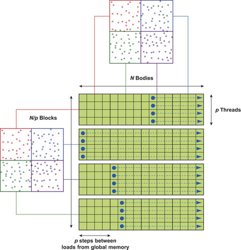 |
| Figure 9.2
Thread block model of the direct evaluation on
gpu
, as in
[24]
.
|
The particle-to-particle (p2p
) interactions of the treecode and
fmm
are calculated in a similar manner (see
Figure 9.3
). The entire domain is decomposed into an oct-tree, and each cell at the leaf level is assigned to a thread block. When the number of particles per cell is larger than the size of the thread block, it is split into multiple thread blocks. The main difference with an all-pairs interaction is that each thread block has a different list of source particles. Thus, it is necessary for each thread block to have its unique index list for the offset of source particles. Only the initial offset (for the cells shown in
Figure 9.3
) is passed to the
gpu
, and the remaining offsets are determined by increments of
 .
.
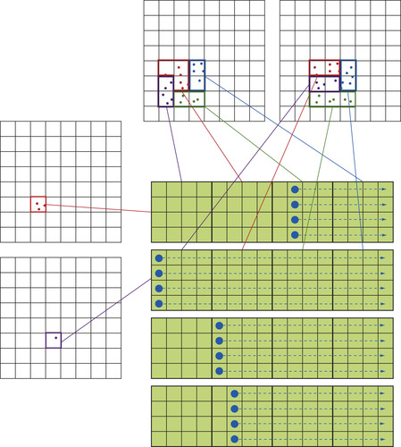 |
| Figure 9.3
Thread block model of the particle-particle interaction on
gpu
s.
|
In order to ensure coalesced memory access, we accumulate all the source data into a large buffer. On the
cpu
, we perform a loop over all interaction lists as if we were performing the actual kernel execution, but instead of calculating the kernel, we store the position vector and mass/charge into one large buffer that is passed on to the
gpu
. This way, the memory access within the
gpu
kernel is always contiguous because the variables are being stored in exactly the same order that they will be accessed. The time it takes to copy the data into the buffer is less than 1% of the entire calculation. Subsequently,
the
gpu
kernel is called, and all the information in the buffer is processed in one call (if it fits in the global memory of the
gpu
). The buffer is split up into an optimum size if it becomes too large to fit on the global memory. We also create a buffer for the target particles, which contains the position vectors. Once they are passed to the
gpu
, the target buffer will be accessed in strides of
 , assigning one particle to each thread. Because the source particle list is different for each target cell (see
Figure 9.3
), having particles from two different cells in one thread block causes branching of the instruction. We avoid this by padding the target buffer, instead of accumulating the particles in the next cell. For example, if there are 2000 particles per box and the thread block size is 128, the target buffer will be padded with 48 particles so that it uses 16 thread blocks of size 128 (
, assigning one particle to each thread. Because the source particle list is different for each target cell (see
Figure 9.3
), having particles from two different cells in one thread block causes branching of the instruction. We avoid this by padding the target buffer, instead of accumulating the particles in the next cell. For example, if there are 2000 particles per box and the thread block size is 128, the target buffer will be padded with 48 particles so that it uses 16 thread blocks of size 128 ( ) for that cell. In such a case, 1 out of the 16 thread blocks will be doing
 excess work, which is an acceptable trade-off to avoid branching of the instruction within a thread block.
The implementation model used for the
p2p
calculation can be applied to all other steps in the
fmm
. An example for the
m2l
translation kernel is shown in
Figure 9.4
. Instead of having particle information in each cell, the cell-cell interactions contain many expansion coefficients per cell. Thus, it is natural to assign one target expansion coefficient to each thread while assigning the cell itself to a thread block.
The typical number of expansion coefficients is in the order of 10-100, and therefore, the padding issue discussed in the previous paragraph has greater consequences for this case. In the simplest
cuda
implementation that we wish to present in this contribution, we simply reduce the thread block size
 to alleviate the problem. In the case of particle-cell interactions (p2m
) or cell-particles interactions (m2p
,
l2p
), the same logic is applied where either the target expansion coefficients or target particles are assigned to each thread, and the source expansion coefficients or source particles are read from the source buffer in a coalesced manner and sequentially processed in strides of
to alleviate the problem. In the case of particle-cell interactions (p2m
) or cell-particles interactions (m2p
,
l2p
), the same logic is applied where either the target expansion coefficients or target particles are assigned to each thread, and the source expansion coefficients or source particles are read from the source buffer in a coalesced manner and sequentially processed in strides of
 .
.
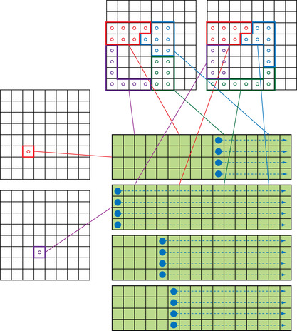 |
| Figure 9.4
Thread block model of the cell-cell interaction on
gpu
s.
|
9.4. Improvements of Performance
We consider the performance of the treecode and
fmm
on
gpu
s for the same model problem as in Nyland
et al.
[24]
. We would like to point out that the performance metrics shown here apply for the very basic and simplified versions of these kernels. The purpose of this contribution is to show the reader how easy it is to write
cuda
programs for the treecode and
fmm
. Therefore, many advanced techniques, which would be considered standard for the expert in these algorithms, are deliberately omitted (see
Section 9.6
). The performance is reported to allow the readers to reproduce the results and verify that their code is performing as expected, as well as to motivate the discussion about the importance of fast algorithms; we do not claim that the kernels here are as fast as they could be. The
cpu
tests were run on an Intel Core i7 2.67 GHz processor, and the
gpu
tests were run on an
nvidia
295
gtx
. The gcc− 4.3 compiler with option −
O3
was used to compile the
cpu
codes and
nvcc
with −
use_fast_math
was used to compile the
cuda
codes.
Figure 9.5
shows the calculation time against the number of bodies for the direct evaluation, treecode, and
fmm
on a
cpu
and
gpu
. The direct calculation is about 300 times faster on the
gpu
, compared with the single-core
cpu
. The treecode and
fmm
are approximately 100 and 30 times faster on the
gpu
, respectively. For
 , the overhead in the tree construction degrades the performance of the
gpu
versions. The crossover point between the treecode and direct evaluation is
, the overhead in the tree construction degrades the performance of the
gpu
versions. The crossover point between the treecode and direct evaluation is
 on the
cpu
and
on the
cpu
and
 on the
gpu
; the crossover point between the
fmm
and direct evaluation is
on the
gpu
; the crossover point between the
fmm
and direct evaluation is
 on the
cpu
and
on the
cpu
and
 on the
gpu
. Note that both for the treecode and
fmm
, the number of particles at the leaf-level of the tree is higher on the
gpu
, to obtain a well-balanced calculation (i.e., comparable time should be spent on the near field and on the far field). The crossover point between the treecode and
fmm
is
on the
gpu
. Note that both for the treecode and
fmm
, the number of particles at the leaf-level of the tree is higher on the
gpu
, to obtain a well-balanced calculation (i.e., comparable time should be spent on the near field and on the far field). The crossover point between the treecode and
fmm
is
 on the
cpu
, but is unclear on the
gpu
, for the range of our tests.
on the
cpu
, but is unclear on the
gpu
, for the range of our tests.
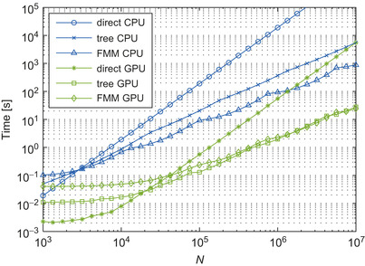 |
| Figure 9.5
Calculation time for the direct method, treecode, and
fmm
on
cpu
and
gpu
. (Normalized
|
When the treecode and
fmm
are performed on the
cpu
, the
p2p
and
m2p
/
m2l
consume more than 99% of the execution time. When these computationally intensive parts are executed on the
gpu
, the execution times of the other stages are no longer negligible. This can be seen in the breakdown shown in
Figure 9.6
for the
 case. The contribution of each stage is stacked on top of one another, so the total height of the bar is the total execution time. The legend on the left and right correspond to the treecode and
fmm
, respectively; “sort” indicates the time it takes to reorder the particles so that they are contiguous within each cell; “other” is the total of everything else, including memory allocation, tree construction, interaction list generation, and so on. The “sort” and “other” operations are performed on the
cpu
. The depth of the tree in this benchmark is the same for both the treecode and
fmm
.
case. The contribution of each stage is stacked on top of one another, so the total height of the bar is the total execution time. The legend on the left and right correspond to the treecode and
fmm
, respectively; “sort” indicates the time it takes to reorder the particles so that they are contiguous within each cell; “other” is the total of everything else, including memory allocation, tree construction, interaction list generation, and so on. The “sort” and “other” operations are performed on the
cpu
. The depth of the tree in this benchmark is the same for both the treecode and
fmm
.
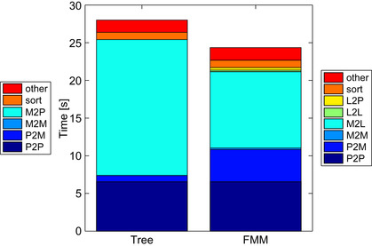 |
| Figure 9.6
Breakdown of the calculation time for the treecode and
fmm
on
gpu
s using
|
As shown in
Figure 9.6
, the
p2p
takes the same amount of time for the treecode and
fmm
. This is due to the fact that we use the same neighbor list for the treecode and
fmm
. It may be worth noting that the standard treecode uses the distance between particles to determine the clustering threshold (for a
given desired accuracy) and has an interaction list that is slightly more flexible than that of the
fmm
. A common measure to determine the clustering in treecodes is the Barnes-Hut multiple acceptance criteria (mac
)
 [3]
, where
[3]
, where
 is the size of the cell, and
 is the distance between the particle and center of mass of the cell. The present calculation uses the standard
fmm
neighbor list shown in
Figure 9.1
for both the
fmm
and treecode, which results in a
mac
of
is the distance between the particle and center of mass of the cell. The present calculation uses the standard
fmm
neighbor list shown in
Figure 9.1
for both the
fmm
and treecode, which results in a
mac
of
 . The
p2m
operation takes longer for the
fmm
because the order of multipole expansions is larger than in the treecode, to achieve the same accuracy. The calculation loads of
m2m
,
l2l
, and
l2p
are small compared with those of
m2p
and
m2l
. The
m2p
has a much larger calculation load than the
m2l
, but it has more data parallelism. Therefore, the
gpu
implementation of these two kernels has a somewhat similar execution time. The high data parallelism of the
m2p
is an important factor we must consider when comparing the treecode and
fmm
on
gpu
s.
. The
p2m
operation takes longer for the
fmm
because the order of multipole expansions is larger than in the treecode, to achieve the same accuracy. The calculation loads of
m2m
,
l2l
, and
l2p
are small compared with those of
m2p
and
m2l
. The
m2p
has a much larger calculation load than the
m2l
, but it has more data parallelism. Therefore, the
gpu
implementation of these two kernels has a somewhat similar execution time. The high data parallelism of the
m2p
is an important factor we must consider when comparing the treecode and
fmm
on
gpu
s.
Figure 9.7
shows the measured performance on the
gpu
, measured in Gflop/s; this is actual operations performed in the code,
i.e.
, a
sqrt
counts 1, and so on. Clearly, for
 the
gpu
is underutilized, but performance is quite good for the larger values of
N
. The
p2p
operation performs very well, achieving in the order of 300 Gflop/s for the larger values of
N
of these tests. The
m2p
performs much better than the
m2l
, owing to the higher inherent parallelism. This explains why we see the treecode accelerating better overall, compared with
fmm
, in
Figure 9.5
.
the
gpu
is underutilized, but performance is quite good for the larger values of
N
. The
p2p
operation performs very well, achieving in the order of 300 Gflop/s for the larger values of
N
of these tests. The
m2p
performs much better than the
m2l
, owing to the higher inherent parallelism. This explains why we see the treecode accelerating better overall, compared with
fmm
, in
Figure 9.5
.
 |
| Figure 9.7
Actual performance in Gflop/s of three core kernels, for different values of
N
.
|
9.5. Detailed Description of the
GPU
Kernels
In this section, we provide a detailed explanation of the implementation of the treecode/
fmm
in
cuda
. The code snippets shown here are extracted directly from the code available from the distribution released with this article.
2
In particular, we will describe the implementation of the
p2p
and
m2l
kernels, which take up most of the calculation time.
2
All source code can be found in
http://code.google.com/p/gemsfmm/
.
9.5.1. The P2P Kernel Implementation
We start with the simplest kernel for the interaction of a single pair of particles, shown in
Listing 9.1
.
Equation 9.1
is calculated here without the
 . In other words, it is the acceleration
 that is
being calculated. This part of the code is very similar to that of the
nbody
example in the
cuda sdk
, which is explained in detail in Nyland
et al.
[24]
. The only difference is that the present kernel uses the reciprocal square-root function instead of a square root and division. There are 19 floating-point operations in this kernel, counting the three additions, six subtractions, nine multiplications, and one reciprocal square root. The list of variables is as follows:
that is
being calculated. This part of the code is very similar to that of the
nbody
example in the
cuda sdk
, which is explained in detail in Nyland
et al.
[24]
. The only difference is that the present kernel uses the reciprocal square-root function instead of a square root and division. There are 19 floating-point operations in this kernel, counting the three additions, six subtractions, nine multiplications, and one reciprocal square root. The list of variables is as follows:
•
posTarget
is the position vector of the target particles; it has a
float3
data type and is stored in registers.
•
sharedPosSource
is the position vector and the mass of the source particles; it has a
float4
data type and resides in shared memory.
•
accel
is the acceleration vector of the target particles; it has a
float3
data type and is stored in registers.
• the
float3
data type is used to store the distance vectors
dist
.
•
eps
is the softening factor
[1]
.
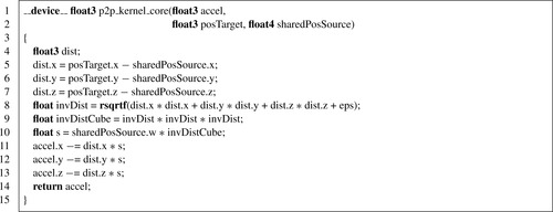 |
| Listing 9.1
p2p
kernel for a single interaction.
|
The function shown in
Listing 9.1
is called from an outer kernel that calculates the pair-wise interactions of all particles in the
p2p
interaction list. This outer kernel is shown in
Listing 9.2
and its graphical representation is shown in
Figure 9.3
. The input variables are
deviceOffset
,
devicePosTarget
, and
devicePosSource
. The output is
deviceAccel
. The description of these variables is as follows:
•
deviceOffset
contains the number of interacting cells and the offset of the particle index for each of these cells.
•
devicePosTarget
contains the position vector of the target particles.
•
devicePosSource
is the position vector of the source particles.
•
deviceAccel
is the acceleration vector of target particles.
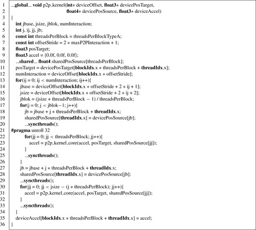 |
| Listing 9.2
The entire
p2p
kernel.
|
All variables that begin with “
device
” are stored in the device memory. All variables that begin with “
shared
” are stored in shared memory. Everything else is stored in the registers. Lines 4–10 are declarations of variables; it is possible to reduce register space usage by reusing some of these variables,
but for pedagogical purposes we have chosen to declare each variable that has a different functionality. There are four variables that are defined externally. One is the
threadsPerBlockTypeA
, which is the number of threads per thread block for the
p2p
kernel. We use a different number of threads per thread block,
threadsPerBlockTypeB
, for the other kernels that have expansion coefficients as targets. On line 5,
threadsPerBlockTypeA
is passed to
threadsPerBlock
as a constant. Another external variable is used on line 7, where
maxP2PInteraction
(the maximum number of neighbor cells in a
p2p
interaction) is used to calculate
offsetStride
(the stride of the data in
deviceOffset
). The other two externally defined variables are
threadIdx
and
blockIdx
, which are thread index and thread-block index provided by
cuda
.
On line 11, the position vectors are copied from the global memory to the registers. On line 12, the number of interacting cells is read from the
deviceOffset
, and on line 13 this number is used
to form a loop that goes through all the interacting cells (27 cells for the
p2p
interaction). Note that each thread block handles (part of) only one target cell, and the interaction list of the neighboring cells is identical for all threads within the thread block. In other words,
blockIdx.x
identifies which target cell we are looking at, and
ij
identifies which source cell it is interacting with. On line 14, the offset of the particle index for that source cell is copied from
deviceOffset
to
jbase
. On line 15, the number of particles in the source cell is copied to
jsize
. Now we have the information of the target particles and the offset and size of the source particles that they interact with. At this point, the information of the source particles still resides in the device memory. This information is copied to the shared memory in coalesced chunks of size
threadsPerBlock
. However, the number of particles per cell is not always a multiple of
threadsPerBlock
, so the last chunk will contain a remainder that is different from
threadsPerBlock
. It is inefficient to have a conditional branching to detect if the chunk is the last one or not, and it is a waste of storage to pad for each source cell. Therefore, on line 16 the number of chunks
jblok
is calculated by rounding up
jsize
to the nearest multiple of
threadsPerBlock
. On line 17, a loop is executed for all chunks except the last one. The last chunk is processed separately on lines 27–33. On line 18, the index of the source particle on the device memory is calculated by offsetting the thread index first by the chunk offset
j*threadsPerBlock
and then by the cell offset
jbase
. On line 19, this global index is used to copy the position vector of the source particles from device memory to shared memory. Subsequently,
__syncthreads()
is called to ensure that the copy to shared memory has completed on all threads before proceeding. On lines 21–24, a loop is performed for all elements in the current chunk of source particles, where the
p2p_kernel_core
is called per pair-wise interaction. The
#pragma unroll 32
is the same loop unrolling suggested in Nyland
et al.
[24]
. On line 25,
__syncthreads()
is called to keep
sharedPosSource
from being overwritten for the next chunk before having been used in the current one. Lines 27–33 are identical to lines 18–25 except for the loop counter for
jj
, which is the remainder instead of
threadsPerBlock
. On line 35, the acceleration vector in registers is copied back to the device memory by offsetting the thread index by
blockIdx.x * threadsPerBlock
.
9.5.2. The M2L Kernel Implementation
As shown in
Equations 9.2
and
9.3
, the multipole-to-local translation in the
fmm
is the translation of the multipole expansion coefficients
 in one location to the local expansion coefficients
 at another. If we relabel the indices of the local expansion matrix to
 , the
m2l
translation can be written as
, the
m2l
translation can be written as
 where
where
 is the imaginary unit,
 is the order of the series expansion,
 is defined as
 and
and
 is the spherical harmonic
(9.4)
(9.5)
(9.6)
In order to calculate the spherical harmonics, the value of the associated Legendre polynomials
 must be determined. The associated Legendre polynomials have a recurrence relation, which requires only the information of
 to start. The recurrence relations and identities used to generate the full associated Legendre polynomial are


(9.7)
(9.8)
(9.9)
The
m2l
kernel calculates
Equation 9.4
in two stages. First,
 is calculated using
Equations 9.5
–
9.9
. Then,
Equation 9.4
is calculated by substituting this result after switching the indices
is calculated using
Equations 9.5
–
9.9
. Then,
Equation 9.4
is calculated by substituting this result after switching the indices
 and
and
 . Thus,
 is calculated at the second stage. Furthermore, in the
gpu
implementation the complex part
is calculated at the second stage. Furthermore, in the
gpu
implementation the complex part
 in
Equation 9.6
is multiplied at the end of the second stage so that the values remain real until then. At the end of the second stage, we simply put the real and complex part of the
in
Equation 9.6
is multiplied at the end of the second stage so that the values remain real until then. At the end of the second stage, we simply put the real and complex part of the
 into two separate variables.
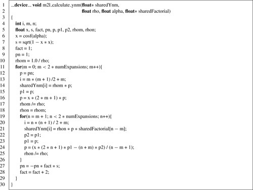
The
gpu
implementation of the first part for
 is shown in
Listing 9.3
. As was the case with
Listing 9.1
, this function is called from an outer function that calculates the entire
m2l
translation for all cells. The inputs are
rho
,
alpha
, and
sharedFactorial
. The output is
sharedYnm
. Because we do not calculate the
is shown in
Listing 9.3
. As was the case with
Listing 9.1
, this function is called from an outer function that calculates the entire
m2l
translation for all cells. The inputs are
rho
,
alpha
, and
sharedFactorial
. The output is
sharedYnm
. Because we do not calculate the
 part of the spherical harmonic at this point,
beta
is not necessary.
sharedFactorial
contains the values of the factorials for a given index;
i.e.
,
sharedFactorial[n]
part of the spherical harmonic at this point,
beta
is not necessary.
sharedFactorial
contains the values of the factorials for a given index;
i.e.
,
sharedFactorial[n]
 . Also, it is
 that is stored in
sharedYnm
and not
that is stored in
sharedYnm
and not
 itself. Basically,
Equation 9.7
is calculated on line 24,
Equation 9.8
is calculated on line 27, and
Equation 9.9
is calculated on line 16.
p
,
p1
, and
p2
correspond to
itself. Basically,
Equation 9.7
is calculated on line 24,
Equation 9.8
is calculated on line 27, and
Equation 9.9
is calculated on line 16.
p
,
p1
, and
p2
correspond to
 ,
,
 , and
, and
 , respectively. However,
p
is used in lines 14 and 21 before it is updated on lines 16 and 24, so it represents
, respectively. However,
p
is used in lines 14 and 21 before it is updated on lines 16 and 24, so it represents
 at the time of usage. This
 is used to calculate
 on lines 14 and 21, although the correspondence to the equation is not obvious at first hand. The connection to the equation will become clear when we do the following transformation,
(9.10)
 |
| Listing 9.3
Calculation of the spherical harmonic for the
m2l
kernel.
|
As mentioned earlier, we do not calculate the
 at this point so
sharedYnm
is symmetric with respect to the sign of
at this point so
sharedYnm
is symmetric with respect to the sign of
 . Therefore, the present loop for the recurrence relation is performed for only
 and the absolute sign for
 in
Equation 9.6
disappears. We can also save shared memory consumption by storing only the
in
Equation 9.6
disappears. We can also save shared memory consumption by storing only the
 half of the spherical harmonic in
sharedYnm
.
half of the spherical harmonic in
sharedYnm
.
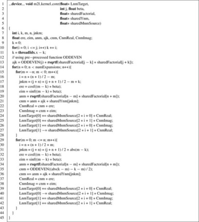
The second stage of the
m2l
kernel is shown in
Listing 9.4
. The inputs are
j
,
beta
,
sharedFactorial
,
sharedYnm
, and
sharedMnmSource
. The output is
LnmTarget
. In this second stage of the
m2l
, the remaining parts of
Equation 9.4
are calculated to obtain
 . Each thread handles a different coefficient in
 . In order to do this, we must associate the
threadIdx.x
to a pair of
j
and
k
. In the outer function, which will be shown later, the index
j
corresponding to
threadIdx.x
is calculated and passed to the present function. Lines 9–11, determine the index
k
from the input
j
and
threadIdx.x
.
. In order to do this, we must associate the
threadIdx.x
to a pair of
j
and
k
. In the outer function, which will be shown later, the index
j
corresponding to
threadIdx.x
is calculated and passed to the present function. Lines 9–11, determine the index
k
from the input
j
and
threadIdx.x
.
 |
| Listing 9.4
Calculation of
|
We will remind the reader again that this part of the
m2l
kernel calculates

 . This results in a quadruple loop over the indices
 ,
,
 ,
,
 , and
, and
 . However, in the
gpu
implementation the first two indices are thread parallelized, only leaving
. However, in the
gpu
implementation the first two indices are thread parallelized, only leaving
 and
and
 as sequential loops
starting from lines 13, 14, and 28. Lines 14–27 are for negative
as sequential loops
starting from lines 13, 14, and 28. Lines 14–27 are for negative
 , while lines 28–42 are for positive
 .
.
 is calculated on line 12. We define a preprocessed function “
#define ODDEVEN(n) ((n & 1 == 1) ? −1: 1)
”, which calculates
is calculated on line 12. We define a preprocessed function “
#define ODDEVEN(n) ((n & 1 == 1) ? −1: 1)
”, which calculates
 without using a power function.
 is calculated on lines 19 and 33.
 is calculated on line 34 for the
 case, and is always
 for
for
 . Because
 is always an even number, it is possible to calculate
 as
as
 and use the
ODDEVEN
function defined previously. Then,
anm
,
ajk
, and
sharedYnm
are multiplied to this result. The complex part
and use the
ODDEVEN
function defined previously. Then,
anm
,
ajk
, and
sharedYnm
are multiplied to this result. The complex part
 that was omitted in the first stage is calculated on lines 17–18 and 31–32 using the index
 instead of
 ;
ere
is the real part and
eim
is the imaginary part.
CnmReal
and
CnmImag
in lines 21–22 and 36–37 are the real and imaginary parts of the product of all the terms previously described. Finally, these values are multiplied to
;
ere
is the real part and
eim
is the imaginary part.
CnmReal
and
CnmImag
in lines 21–22 and 36–37 are the real and imaginary parts of the product of all the terms previously described. Finally, these values are multiplied to
 in lines 23–26 and 38–41, where
sharedMnmSource[2*i+0]
is the real part and
sharedMnmSource[2*i+1]
is the imaginary part. We use the relation
in lines 23–26 and 38–41, where
sharedMnmSource[2*i+0]
is the real part and
sharedMnmSource[2*i+1]
is the imaginary part. We use the relation
 to reduce the storage of
sharedMnmSource
. Therefore, the imaginary part has opposite signs for the
to reduce the storage of
sharedMnmSource
. Therefore, the imaginary part has opposite signs for the
 case and
 case. The real part of
 is accumulated in
LnmTarget[0]
, while the imaginary part is accumulated in
LnmTarget[1]
.
is accumulated in
LnmTarget[0]
, while the imaginary part is accumulated in
LnmTarget[1]
.
The functions in
Listing 9.3
and
Listing 9.4
are called from an outer function shown in
Listing 9.5
. This function is similar to the one shown in
Listing 9.2
. The inputs are
deviceOffset
and
deviceMnmSource
. The output is
deviceLnmTarget
. The definitions are:
•
deviceOffset
contains the number of interacting cells, the offset of the particle index for each of these cells, and the 3D index of their relative positioning;
•
threadsPerBlockTypeB
and
maxM2LInteraction
are defined externally;
•
maxM2LInteraction
is the maximum size of the interaction list for the
m2l
, which is 189 for the present kernels; and
•
offsetStride
, calculated on line 6, is the stride of the data in
deviceOffset
.
 |
| Listing 9.5
The entire
m2l
kernel.
|
On line 8, the size of the cell is read from
deviceConstant[0]
, which resides in constant memory. On line 10,
LnmTarget
is initialized. Each thread handles a different coefficient in
 . In order to do this, we must associate the
threadIdx.x
to a pair of
j
and
k
.
sharedJ
returns the index
. In order to do this, we must associate the
threadIdx.x
to a pair of
j
and
k
.
sharedJ
returns the index
 when given the
threadIdx.x
as input. It is declared on line 11 and initialized on lines 16–18. The values are calculated on lines 19–24, and then passed to
m2l_kernel_core()
on line 40.
sharedMnmSource
is the copy of
deviceMnmSource
in shared memory. It is declared on line 12 and the values are copied on lines 35–36 before it is passed to
m2l_kernel_core()
on line 41.
sharedYnm
contains the real spherical harmonics. It is declared on line 13, and its values are calculated in the function
m2l_calculate_ynm
on line 39 before they are passed to
m2l_kernel_core
on line 41.
sharedFactorial
contains the factorial for the given index and is declared on line 14 and its values are calculated on lines 25–29 before they are passed to
m2l_kernel_core
on line 41. On line 15, the number of interacting cells is read from
deviceOffset
and its value
numInteraction
is used for the loop on line 30. The offset of particles is read from
deviceOffset
on line 31, and the relative distance of the source and target cell is calculated on lines 32–34. On line 38, this distance is transformed into spherical coordinates using an externally defined function
cart2sph
. The two functions shown in
Listing 9.3
and
Listing 9.4
are called on lines 39–41. Finally, the results in
LnmTarget
are copied to
deviceLnmTarget
on line 45.
when given the
threadIdx.x
as input. It is declared on line 11 and initialized on lines 16–18. The values are calculated on lines 19–24, and then passed to
m2l_kernel_core()
on line 40.
sharedMnmSource
is the copy of
deviceMnmSource
in shared memory. It is declared on line 12 and the values are copied on lines 35–36 before it is passed to
m2l_kernel_core()
on line 41.
sharedYnm
contains the real spherical harmonics. It is declared on line 13, and its values are calculated in the function
m2l_calculate_ynm
on line 39 before they are passed to
m2l_kernel_core
on line 41.
sharedFactorial
contains the factorial for the given index and is declared on line 14 and its values are calculated on lines 25–29 before they are passed to
m2l_kernel_core
on line 41. On line 15, the number of interacting cells is read from
deviceOffset
and its value
numInteraction
is used for the loop on line 30. The offset of particles is read from
deviceOffset
on line 31, and the relative distance of the source and target cell is calculated on lines 32–34. On line 38, this distance is transformed into spherical coordinates using an externally defined function
cart2sph
. The two functions shown in
Listing 9.3
and
Listing 9.4
are called on lines 39–41. Finally, the results in
LnmTarget
are copied to
deviceLnmTarget
on line 45.
Listing 9.1
Listing 9.2
Listing 9.3
Listing 9.4
and
Listing 9.5
are the core components of the present
gpu
implementation. We hope that the other parts of the open-source code that we provide along with this article are understandable to the reader without explanation.
9.6. Overview of Advanced Techniques
There are various techniques that can be used to enhance the performance of the treecode and
fmm
. The
fmm
presented in this article uses the standard translation operator for translating multipole/local expansions. As the order of expansion
 increases, the calculation increases as
 for this method. There are alternatives that can bring the complexity down to
 [5]
or even
[5]
or even
 [14]
. In the code that we have released along with this article, we have included an implementation of the
[14]
. In the code that we have released along with this article, we have included an implementation of the
 translation kernel by
[5]
as an extension. We have omitted the explanations in this text, however, and consider the advanced reader able to self-learn the techniques from the literature to understand the code. Some other techniques that can improve the performance are the optimization of the order of expansion for each interaction
[7]
, the use of a more efficient
m2l
interaction stencil
[15]
and the use of a treecode/
fmm
hybrid, as suggested in
[5]
. It is needless to mention that the parallelization of the
code for multi-
gpu
calculations
[17]
and
[18]
is an important extension to the treecode/
fmm
on
gpu
s. Again, this is an advanced topic beyond the scope of this contribution.
translation kernel by
[5]
as an extension. We have omitted the explanations in this text, however, and consider the advanced reader able to self-learn the techniques from the literature to understand the code. Some other techniques that can improve the performance are the optimization of the order of expansion for each interaction
[7]
, the use of a more efficient
m2l
interaction stencil
[15]
and the use of a treecode/
fmm
hybrid, as suggested in
[5]
. It is needless to mention that the parallelization of the
code for multi-
gpu
calculations
[17]
and
[18]
is an important extension to the treecode/
fmm
on
gpu
s. Again, this is an advanced topic beyond the scope of this contribution.
When you are reporting the
gpu
/
cpu
speedup, it is bad form to compare the results against an un-optimized serial
cpu
implementation. Sadly, this is often done, which negatively affects the credibility of results in the field. For this contribution, we have used a reasonable serial code in
c
, but it is certainly not so fast as it could be. For example, it is possible to achieve over an order of magnitude performance increase on the
cpu
by doing single-precision calculations using
sse
instructions with inline assembly code
[23]
. For those who are interested in the comparison between a highly tuned
cpu
code and highly tuned
gpu
code, we provide a highly tuned
cpu
implementation of the treecode/
fmm
in the code package that we release with this book.
9.7. Conclusions
This contribution is a follow-on from the previous
GPU Gems 3
, Chapter 31
[24]
, where the acceleration of the all-pairs computation on
gpu
s was presented for the case of the gravitational potential of
N
masses. We encourage the reader to consult that previous contribution, as it will complement the presentation we have given. As can be seen in the results presented here, the cross-over point where fast
N
-body algorithms become advantageous over direct, all-pairs calculations is in the order of
 for the
cpu
and in the order of
for the
cpu
and in the order of
 for the
gpu
. Hence, utilizing the
gpu
architecture moves the cross-over point upward by one order of magnitude, but this size of problem is much smaller than many applications require. If the application of interest involves, say, millions of interacting bodies, the advantage of fast algorithms is clear, in both
cpu
and
gpu
hardware. With our basic kernels, about
for the
gpu
. Hence, utilizing the
gpu
architecture moves the cross-over point upward by one order of magnitude, but this size of problem is much smaller than many applications require. If the application of interest involves, say, millions of interacting bodies, the advantage of fast algorithms is clear, in both
cpu
and
gpu
hardware. With our basic kernels, about
 speedup is obtained from the fast algorithm on the
gpu
for a million particles. For
speedup is obtained from the fast algorithm on the
gpu
for a million particles. For
 , the fast algorithms provide
 speedup over direct methods on the
gpu
. However, if the problem at hand requires small systems, smaller than
speedup over direct methods on the
gpu
. However, if the problem at hand requires small systems, smaller than
 , say, one would be justified to settle for the all-pairs, direct calculation.
The main conclusion that we would like the reader to draw from this contribution is that constructing fast
N
-body algorithms on the
gpu
is far from a formidable task. Here, we have shown basic kernels that achieve substantial speedup over direct evaluation in less than 200 lines of
cuda
code. Expert-level implementations will, of course, be much more involved and would achieve more performance. But a basic implementation like the one shown here is definitely worthwhile.
We thank F. A. Cruz for various discussions that contributed to the quality of this chapter.
References
[1]
S. Aarseth,
Gravitational N-Body Simulations
. (2003
)
Cambridge University Press
,
Cambridge, United Kingdom
.
[2]
M.S. Bapat, L. Shen, Y.J. Liu,
An adaptive fast multipole boundary element method for three-dimensional half-space acoustic wave problems
,
Eng. Anal. Bound. Elem.
33
(8–9
) (2009
)
1113
–
1123
.
[3]
J. Barnes, P. Hut,
A hierarchical
O
(N
log
N
) force-calculation algorithm
,
Nature
449
(1986
)
324
–
446
.
[4]
J.A. Board Jr., J.W. Causey, J.F. Leathrum Jr., A. Windemuth, K. Schulten,
Accelerated molecular dynamics simulation with the parallel fast multipole algorithm
,
Chem. Phys. Lett.
198
(1–2
) (1992
)
89
–
94
.
[5]
H. Cheng, L. Greengard, V. Rokhlin,
A fast adaptive multipole algorithm in three dimensions
,
J. Comput. Phys.
155
(1999
)
468
–
498
.
[6]
E. Darve, P. Have,
Efficient fast multipole method for low-frequency scattering
,
J. Comput. Phys.
197
(2004
)
341
–
363
.
[7]
H. Daschel,
Corrected article: an error-controlled fast multipole method
,
J. Chem. Phys.
132
(2010
)
119901
.
[8]
K.C. Donepudi, J.-M. Jin, W.C. Chew,
A higher order multilevel fast multipole algorithm for scattering from mixed conducting/dielectric bodies
,
IEEE Trans. Antennas Propag.
51
(10
) (2003
)
2814
–
2821
.
[9]
F. Ethridge, L. Greengard,
A new fast-multipole accelerated Poisson solver in two dimensions
,
SIAM J. Sci. Comput.
23
(3
) (2001
)
741
–
760
.
[10]
H. Fujiwara,
The fast multipole method for integral equations of seismic scattering problems
,
Geophys. J. Int.
133
(1998
)
773
–
782
.
[11]
L. Gorelick, M. Galun, E. Sharon, R. Basri, A. Brandt,
Shape representation and classification using the Poisson equation
,
IEEE Trans. Pattern Anal. Mach. Intell.
28
(2006
)
1991
–
2005
.
[12]
L. Greengard, J.-Y. Lee,
A direct adaptive Poisson solver of arbitrary order accuracy
,
J. Comp. Phys.
125
(1996
)
415
–
424
.
[13]
L. Greengard, V. Rokhlin,
A fast algorithm for particle simulations
,
J. Comput. Phys.
73
(2
) (1987
)
325
–
348
.
[14]
N.A. Gumerov, R. Duraiswami,
Fast Multipole Methods for the Helmholtz Equation in Three Dimensions
.
first ed.
(2004
)
Elsevier Ltd.
,
Oxford
.
[15]
N.A. Gumerov, R. Duraiswami,
Fast multipole methods on graphics processors
,
J. Comp. Phys.
227
(18
) (2008
)
8290
–
8313
.
[16]
N.A. Gumerov, R. Duraiswami,
A broadband fast multipole accelerated boundary element method for the three dimensional Helmholtz equation
,
J. Acoust. Soc. Am.
125
(1
) (2009
)
191
–
205
.
[17]
T. Hamada, T. Narumi, R. Yokota, K. Yasuoka, K. Nitadori, M. Taiji,
42 TFlops hierarchical N-body simulations on GPUs with applications in both astrophysics and turbulence
,
In:
Proceedings of the Conference on High Performance Computing Networking
November 2009, Portland OR, Storage and Analysis, SC ’09
. (2009
)
ACM
,
New York
, pp.
1
–
12
.
[18]
I. Lashuk, A. Chandramowlishwaran, H. Langston, T.-A. Nguyen, R. Sampath, A. Shringarpure,
et al.
,
A massively parallel adaptive fast-multipole method on heterogeneous architectures
,
In:
Proceedings of the Conference on High Performance Computing Networking
November 2009, Portland OR, Storage and Analysis, SC ’09
. (2009
)
ACM
,
New York, NY
, pp.
1
–
12
.
[19]
Y.J. Liu, N. Nishimura,
The fast multipole boundary element method for potential problems: a tutorial
,
Eng. Anal. Bound. Elem.
30
(2006
)
371
–
381
.
[20]
Y. Liu,
Fast Multipole Boundary Element Method: Theory and Applications in Engineering
. (2009
)
Cambridge University Press
,
Cambridge, United Kingdom
.
[21]
H. Nguyen, GPU Gems 3, Addison-Wesley Professional, 2007, Available from:
http://developer.nvidia.com/object/gpu-gems-3.html
.
[22]
N. Nishimura,
Fast multipole accelerated boundary integral equation methods
,
Appl. Mech. Rev.
55
(4
) (2002
)
299
–
324
.
[23]
K. Nitadori, K. Yoshikawa, J. Makino, Personal Communication.
[24]
L. Nyland, M. Harris, J. Prins,
Fast
N
-body simulation with CUDA
,
In:
GPU Gems
,
3
(2007
)
Addison-Wesley Professional
, pp.
677
–
695
;
(Chapter 31)
.
[25]
V. Rokhlin,
Rapid solution of integral equations of scattering theory in two dimensions
,
J. Comp. Phys.
86
(2
) (1990
)
414
–
439
.
[26]
C. Sagui, A. Darden,
Molecular dynamics simulations of biomolecules: long-range electrostatic effects
,
Annu. Rev. Biophys. Biomol. Struct.
28
(1999
)
155
–
179
.
..................Content has been hidden....................
You can't read the all page of ebook, please click here login for view all page.