
Chapter 12. Massive Parallel Computing to Accelerate Genome-Matching
Ben Weiss and Mike Bailey
This chapter explores the process of defining and optimizing a relatively simple matching algorithm in CUDA. The project was designed to be a tool to explore the process of developing algorithms from start to finish with CUDA in mind; it also intended to highlight some of the differences between development in a massively parallel GPU-based architecture and a more traditional CPU-based single- or multi- threaded one. Framed in the context of a real-world genetic sequence alignment problem, we explored and quantified the effect of various attempts to speed up this code, ultimately achieving more than two orders of magnitude of improvement over our original CUDA implementation and over three orders of magnitude of improvement over our original CPU version.
12.1. Introduction, Problem Statement, and Context
Because exploration and learning were the primary goals, we chose to explore the development of a solution to a well-understood computational genetics problem that seeks to align short sequences of genetic material against a larger fully sequenced genome or chromosome. This choice originated with a desire to support Michael Freitag's (Oregon State University) genetics research. This provided a real-world customer with real datasets and requirements. However, in the broader aspect, the lessons learned throughout the development of this code will act as a guide to anyone trying to write any high-efficiency comparison algorithms on CUDA, beyond computational genetics. Our hope is that the lessons we learned can save others time and effort in understanding at least one way of using and optimizing for the CUDA platform. We attempt to present the give and take between optimizing the algorithm and tweaking the problem statement itself to better suit the CUDA platform; several of our most significant improvements came as we rephrased the problem to more accurately suit CUDA's abilities within the context of our customers’ needs.
As sequencing machines produce larger and larger datasets, the computational requirements of aligning the reads into a reference genome have become increasingly great
[8]
. Modern sequencing machines can produce batches of millions of short (< 100 base pair) reads, here referred to as “targets” for clarity, which need to be aligned against a known reference genome. Several CPU-based solutions
have been developed to address this issue, a few of which have been ported to CUDA, but we chose instead to present a method developed with CUDA in mind from the very beginning. A small snippet of pseudo code (Listing 12.1
) and an illustrative graphic (Figure 12.1
) provide a naive solution that clarifies the fundamental problem that we have solved.
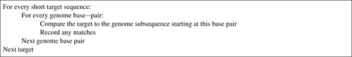 |
| Listing 12.1
Basic problem pseudo code.
|
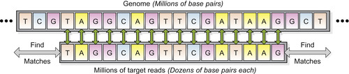 |
| Figure 12.1
Illustration of the basic problem being solved. A large genome is searched for matches to a long list of target reads.
|
This problem appeared to be a good match for implementation in CUDA because the code is highly parallelizable and fits well into an Single Instruction, Multiple Data (SIMT) paradigm. Additionally, the cost-effectiveness of using NVIDIA hardware to solve this problem made a CUDA solution appealing: a traditional cluster could have cost 10 times what an equivalent desktop GPU solution might cost. Hashing the genome and target sequences, one of the standard techniques for solving a problem like this, was implemented very late in the development of our solution in part because it complicates the algorithm's data access patterns significantly and makes it more difficult to optimize.
For the development phase of our specific algorithm, a benchmark set of 5000 real-world 36 base pair (BP) targets (reads) was replicated many times and matched against an already-sequenced map of linkage group VII of
Neurospora crassa
(3.9 million BP). This was used as a baseline to gauge the performance of the algorithm, which had to run on inexpensive hardware and scale to problems with millions or even billions of reads and tens of millions of genome base pairs.
12.2. Core Methods
The algorithm presented here, which currently reports only exact matches of the target reads onto the references genome, differs significantly in structure from many previously available codes because
instead of seeking to port a CPU-centric algorithm to the GPU, we built the solution entirely with CUDA 1.1 in mind. In this section, we present a brief overview of our comparison kernel.
The first few steps of each kernel involved rearranging memory on the GPU. Though somewhat mundane, these tasks received a great deal of time in the optimization process because the various memory access pathways and caches available in CUDA are strikingly different than the cache layers of a CPU. First, a section of genome was loaded from global memory into shared memory; this section of genome persisted throughout the comparison operation. The load operation was designed to create a series of coalesced memory transfers that maximized speed, and each block takes a different section of the genome.
Next, each thread loaded a target into a different section of shared memory. In each kernel, all blocks checked the same series of several thousand targets, so targets were stored in constant memory to take advantage of on-chip caching. Once loaded, each thread checked its target against the portions of the genome stored locally in each block's shared memory, recording matches in a global memory array. After a target had been checked, a new one was loaded from constant memory to replace it, and the comparison repeated until all designated targets had been handled. In successive kernel calls, the constant memory was reloaded with new targets.
A simple example clarifies the process. Suppose we have a short section of genome and a list of four targets that we match using a kernel with two blocks and three threads per block (see
Figure 12.2
). First, each block loads a section of genome into shared memory; then each thread grabs a target and compares it against the cached portion of the genome. Most threads do not find matches, but thread 3 in block 1 does, and records the target identifier and genome offset in global memory. When the first three targets have been handled, the next three are loaded and checked. All matches are recorded. The process continues until all targets for the run have been handled. Of course, CUDA does this with dozens of threads in hundreds of blocks at a time.
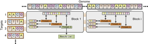 |
| Figure 12.2
Example of a kernel of three threads doing a comparison.
|
Late in the development of the algorithm, a hash table was implemented, sorting each genome offset and target based on the first eight BPs. This, vaguely similar to Maq's seed index table
[7]
,
[2]
, allows the algorithm to consider only genome/target matches where the first few base pairs already match, increasing the probability by several orders of magnitude that a comparison will succeed. Most commercial CPU-based alignment algorithms use a hash table of some form. No advantage was gained
by computing target reverse-complements on the fly, so when enabled, complements are precomputed on the CPU and added to the target list.
In addition to the CUDA kernel, a multithreaded CPU version was built with a similar formulation, though organized and optimized somewhat differently to cater to the differences between the architectures, especially in the way that memory is allocated and arranged. Details of these differences are discussed later in this chapter. Running both CPU and CUDA versions of the comparison in parallel provided still greater speed, but also presented additional challenges.
In the following sections, we will explore some of the specific changes made, but major lessons learned are summarized here. As expected, multiprocessor occupancy was found to be important, though on more recent hardware this parameter is easier to keep high because of increases in the number of available registers in each multiprocessor. Additionally, optimizing and utilizing the various memory pathways are critical for this kind of high-throughput code. In order to maximize these indicators of performance, both algorithm design and kernel parameter settings must be carefully selected. Also as expected, wrap cohesion was found to be important, but if the basic kernel flow is cohesive, the NVCC compiler handles this without much need for programmer involvement.
With its complex memory pathways and computation architecture, CUDA is fundamentally different than the CPU for performance applications, and one should approach CUDA carefully, with the understanding that some conventional wisdom from single-threaded programming does not work in an SIMT environment.
12.3. Algorithms, Implementations, and Evaluations
A main goal of the project was to determine the characteristics of CUDA algorithms that have the greatest influence on execution speed. Thus, our improvements in performance were measured against previous versions of the same code, not the results of other researchers’ solutions, to allow for quantification of the effectiveness of algorithmic changes in increasing efficiency. Most industry-standard codes for this kind of problem support mismatches between target reads and a reference genome, as well as gaps of a few BPs.
Our development occurred on a Pentium 4 3.0 GHz dual-core system with 2 GB of RAM running a single 256 MB GeForce 8600 graphics card, Windows XP Professional, and CUDA 1.1. All performance statistics reported here were based on this system, but we expect that they would scale very well to the newer, faster generations of NVIDIA hardware available.
Throughout the development of the code, the speed improvements and their associated algorithmic changes were carefully tracked to give us an idea of the effectiveness of various strategies in speeding up CUDA code (see
Figure 12.3
). “Targets per second” is representative of the number of targets processed per second during the comparison stage of the algorithm; setup and post-processing time were assumed to be small compared with the computation time for real-world problems, and this metric provided a more direct measure of the performance of the algorithm, rather than the system, making performance improvements in CUDA easier to distinguish.
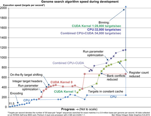 |
| Figure 12.3
Genome search algorithm speed during development, for two different versions of the CUDA kernel and the optimized CPU version of the same algorithm. Points represent significant changes made to the code.
|
Some changes involved optimizations to the code itself while retaining the overall structure of the algorithm; others pertained to changes in the way the problem was solved or (in a few cases) a modification of the problem statement itself. This seems typical of any project developed in CUDA and shows the interplay between the hardware's capabilities and the software's requirements as they
relate to overall speed. In the following sections, we describe some of the most interesting and effective optimizations that we employed.
12.3.1. Genome Encoding
Obviously, reading genetic data in 8-bit ASCII character format is a significant waste of space. Encoding the A's, C's, T's, and G's into a more compact form provided a significant speedup: With each base pair requiring only two bits, four could be packed into each byte and compared at once. Though easily implemented, an algorithmic problem presented itself: The bytes of genome and target data lined up only one-quarter of the time. To resolve this we created four “subtargets” for every target sequence (read), each with a different sub-byte offset, and introduced a bitwise mask to filter out the unused BPs in any comparison. All told, this change (which occurred while still investigating the problem on the CPU before initial implementation in CUDA) improved performance only by about 10%, but
significantly reduced memory usage and paved the way for more effective changes. Although search algorithms in other disciplines may not have such an obvious encoding scheme, this result still indicates that for high-throughput applications like this, packing the relevant data even though it consumes a bit more GPU horsepower can provide a significant speedup.
Figure 12.4
demonstrates the compression and masking process.
 |
| Figure 12.4
A switch from single BP compares to encoded BPs comparing whole bytes at a time. When the genome and target don't align at byte boundaries, a mask filters out the unused base pairs.
|
12.3.2. Target Headers
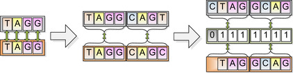
Another inherent inefficiency was addressed: The code runs on a 32-bit multiprocessor, but all comparisons were single-byte operations. Very significant speed gains were made by encoding the genome into
char
arrays and then typecasting them to integers to more fully utilize the pipeline width. In this revision, “headers” were created for each subtarget, containing 4-byte (16-BP) integer versions of the target itself and the accompanying mask, and then the appropriate section of genome was typecast to
int
and compared with the header. Used as a pre-filter for the remainder of the comparison process, this reduced the likelihood of a target passing the header check but not being an actual match to about one in 50 million compares on our test dataset. The result was a speed increase of more than 25% in CPU mode, slightly less under CUDA, which complicates typecasting of
char
to
int
because of its shared memory layout.
Figure 12.5
illustrates a 2-byte target header in action.
 |
| Figure 12.5
A target header in action. If the 16-bit (8 BP) header comparison succeeds, then the compare operation proceeds.
|
Our CUDA kernel stores the genome in shared memory. Shared memory is arranged in 16 banks, each 32 bits wide
[5]
. Presumably because of this unique layout, the NVCC compiler behaves in an unusual way when typecasting from
char
arrays to
int
. When an address for an
int
lies on an even multiple of four bytes, the typecast proceeds as expected. However, when the address is not aligned this
way, the word returned is the next-lowest aligned
int
to the address requested. For example, given an array
char q[8]
that spans two banks:
0xAABBCCDD
is stored in Bank 1 and
0xEEFF1122
in Bank 2, we try the typecast
*(int*)(q + 2)
, which we expect to return
0x1122AABB
. We instead obtain
0xAABBCCDD
— the contents of Bank 1. This makes some sense: The compiler requests memory from one bank at a time to maximize speed, and this fringe case occurs very seldom in practice. However, it extends to other typecasts as well — if a
char
array is typecast to
shorts
, only typecasts to even-numbered bytes give the expected result. Compensating for this behavior requires bit fiddling two bank-aligned integers into the desired portion of the encoded genome for comparison and reduces performance gains significantly. Once we understood this, working with it was not a problem.
12.3.3. Data Layout
Even though CUDA is fundamentally a stream-processing engine, the best access patterns for this kind of problem appeared more like a spider web: The many available memory pathways made moving data around a complex task with easily overlooked subtleties.
Table 12.1
provides an overview of where the data structures needed by the algorithm were stored. Because the comparison mask was fixed, we stored that information in constant memory, which was heavily cached, while the genome resided in global memory and was copied into shared (local) memory for comparison. The entire target list is kept in global memory, but because each kernel uses relatively few targets, a subset is copied to the remaining constant memory for each kernel. Targets are then further cached in shared memory for each compare operation. The texture memory pathway was initially unused, then later pressed into service for loading target and genome hash information, which attempts to take advantage of its spatial locality caching.
The advantage of pulling from different memory sources is a smaller utilization of global memory bandwidth, decreasing the load on one of the weakest links in data-intensive CUDA kernels like ours. On the CPU, however, experiments indicated that the highest speed could be provided by actually replicating the mask set many times and interleaving the target data so that target headers and their associated masks are very close together. Placing the masks in their own array, even though it means almost half as much data is streamed into and out of the CPU, actually slows performance down very significantly (a 35% speed increase for the interleaved scheme).
CUDA's shared memory is arranged in banks capable of serving only one 4-byte word every two clock cycles
[5]
. Successive 32-bit
ints
of shared memory are stored in successive banks, so word 1 is stored in bank 1, word 2 in bank 2, and so on. The importance of understanding this layout was driven home in one design iteration that had the targets arranged in 16-byte-wide structures. Every iteration in all 32 threads read just the first word (the header) from the structure, which resided in only four banks and created an eight-way “bank conflict” — it took 16 GPU clock cycles to retrieve all the data and continue. To alleviate this problem, the target headers were segregated in their own block of shared memory so that every bank was used on every read and presented at most a two-way bank conflict per iteration. This change alone gave us a 35% speed increase.
Each CUDA multiprocessor on the GeForce 8600 graphics card that we used has only 8192 registers, although later architectures have more. This meant that the number of registers a given thread used was very important (a block of 256 threads all wanting 24 registers requires 256 × 24 = 6114 registers, so only one block would be able to execute at a time). A variety of efforts were made to reduce the number of registers in use in the program, the most successful of which involved passing permutations on kernel parameters as additional kernel parameters instead of using extra registers to compute them. Generally, though, the NVCC compiler seemed to do a good job of optimizing for low register count where possible, and almost nothing we tried successfully reduced the number further.
12.3.4. Target Processing
Because so little time is required to do a simple comparison operation, the algorithm was bottlenecked in the global memory bus. A significant performance increase was obtained by creating the subtargets (sub-byte shifts of targets to compensate for the encoding mechanism discussed earlier in this chapter) on the fly on the GPU instead of pregenerating them on the CPU and then reading them in. On the CPU, of course, the extra steps were a significant drain;
not
doing on-the-fly shifting increased performance by roughly 30%. On CUDA,
doing
on-the-fly preprocessing increased performance by about 3% initially, with much more significant benefit later owing to the decreased memory bandwidth involved in moving only one-quarter as much target data into local shared memory.
12.3.5. CUDA Kernel Parameter Settings
The single most significant change in the development of the CUDA version of the algorithm occurred when the kernel parameters (threads per block, targets per kernel, and cache size per block) were first optimized. To do this, a massive systematic search of the entire kernel parameter space was made, seeking a global optimum operating point. The resulting optimum parameters are listed in
Table 12.2
.
| Threads/block | 64 |
| Shared cache size | 7950 bytes/block |
| Blocks/kernel | 319 |
Great care needs to be exercised when selecting these options for a number of reasons. First, there are limited amounts of cache and registers available to each multiprocessor, so setting threads/block
or cache size too large can result in processors having to idle because memory resources are taxed. Additionally, the overhead required to get each block started incurred a penalty for blocks that do too little work, so very small blocks are not advisable. Finally, if blocks ran too long, the OS watchdog timer interfered with execution and manually yanked back control, crashing the kernel and providing impetus to keep blocks/kernel relatively small. One aid we used in setting these parameters was the CUDA Occupancy Calculator, which predicts the effects of execution parameters on GPU utilization
[4]
. The advice of this calculator should be taken with a grain of salt, however, as it cannot know how parameter changes affect the speed of the code itself within each block, but it provides a good indication of how fully the device is being utilized.
12.3.6. Additional Smaller Threads
Midway through the project, the CUDA kernel underwent a significant overhaul (the difference between Kernel 0 and Kernel 1 in
Figure 12.3
). The biggest change came from a desire to reduce the workload of each individual thread. Additional, smaller threads tend to perform better in CUDA, especially if each thread is linked to a proportionate amount of shared memory — the smaller the task, the less shared memory it requires, and the more threads can run. In Kernel 1, targets and subtargets were cached in shared memory, so having each thread do just one subtarget instead of an entire target resulted in a very significant speedup in the long term. Eventually, however, genome hashing forced Kernel 1 to be changed back to one target per thread because the genome locations for successive comparisons were not consecutive.
12.3.7. Combined CUDA and CPU Execution
Using both CUDA and the CPU version of the algorithm seemed like a logical next step, and indeed, doing this improved performance. Some issues became apparent, however, in the loop that waits for CUDA to finish. Out of the box, CUDA is set up to “hot idle” the CPU until the kernel is done, keeping CPU usage at 100% and prohibiting it from doing other tasks. To mitigate this, we used a different approach that queried the device for kernel completion only once every 2–6 ms, using the rest of the time to run comparisons with the CPU version of the algorithm. In this mode, both CPU and GPU see a slight performance hit, but the combined totals still outweigh either individually in our development dataset.
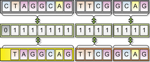
12.3.8. Gaps and Mismatches
Commercial implementations of the short read genome matching problem allow a set number of mismatches between the target and the genome match location, as well as “gaps” — regions of code
inserted in either the genome or the target before the match continues (see
Figure 12.6
). A little binary trickery
[1]
allowed mismatches to be implemented beyond the 16 BP header region with only a slight performance hit. However, to find mismatches in the target header with hashing enabled, all targets would need to be requeried using a header and hash key from a different part of the target (see
Figure 12.6
). This would require all targets to be compared twice to find a mismatch, once for each header, and would reduce performance by more than 50%. This feature has not yet been fully implemented, and so is not reported in any other results, but the fundamental challenges have been overcome. The current code also does not yet support gaps, but once multiple headers for mismatches are in place, it simply makes the comparison operation more complex, reducing performance by an unpleasant, but tolerable, measure.
 |
| Figure 12.6
Example of a compare operation containing a gap and a mismatch.
|
12.3.9. Genome/Target Hashing
The greatest single performance improvement throughout the development of the algorithm came when the genome was hashed into bins, with each bin containing a list of offsets where the sequence matches the same first eight base pairs. This approach is taken by the majority of commercial solutions to this problem, and for good reason. Once targets were similarly binned, only compare operations in the same bin needed to be executed, reducing the total number of comparison operations 2
16
-fold. Information about the genome offsets for each bin was given to the kernel in a texture, utilizing the GPU's cache locality to try to ensure that the next offset needed was readily available in cache. Even just a crude first-round implementation of this feature increased performance by nearly 10x, though the hashing process (which is actually quite quick) was treated as a preprocess, and thus is not included in the performance metrics in
Figure 12.3
.
12.3.10. Scaling Performance
In order to gauge how well this solution scales to larger problems, we tested the algorithm against two real-world datasets that push our GeForce 8600's memory resources to their limit. In each case, wild cards (“N"s) within the genome were ignored, and targets were required to contain no wild cards. The first dataset uses our development test genome (used to create
Figure 12.3
), Linkage Group VII from the sequenced
Neurospora crassa
genome, and searches a target list of slightly more than 3.4 million 36 base-pair segments. The second dataset consists of the first 5.0 million base pairs of chromosome 1 of
N. crassa
and a list of 1.0 million 76 base-pair targets.
Table 12.3
shows the compare times with the most recent version of the algorithm running in CUDA-only mode as well as both CUDA and CPU combined. For reference, one run of the first dataset was limited to only 1.0 million base pairs as well.
| *
Linkage group VII of Neurospora crassa.
| |||||||
| +
First 5 MBP of chromosome 1 of Neurospora crassa.
| |||||||
| Dataset | Genome BP | Target Count | Target Length (BP) | Compare Time (CUDA) | Targets/Second (CUDA) | Compare Time (Both) | Targets/Second (Both) |
|---|---|---|---|---|---|---|---|
| 1 * | 3,938,688 | 1,000,000 | 36 | 24.7 s | 40,400 | 9.7 s | 103,000 |
| 1 * | 3,938,688 | 3,419,999 | 76 | 48.2 s | 70,900 | 22.3 s | 153,000 |
| 2 + | 5,000,000 | 1,000,000 | 76 | 62.2 s | 16,100 | 38.8 s | 25,800 |
These numbers appear significantly higher than the numbers reported in
Figure 12.3
because of the comparatively few exact matches present in these datasets, which reduces the number of expensive writes to global memory. This is to be expected for this application.
12.4. Final Evaluation and Validation of Results, Total Benefits, and Limitations
Our application provided an excellent platform to explore the tuning characteristics of this relatively new computing platform. Much was learned about memory access and kernel execution parameters, which are sensitive aspects of CUDA programs that differ significantly from traditional CPU design problems, but can both have a large impact on performance.
Even after over a year of development, we believe that the algorithm is still far from optimized and that more performance gains can still be expected. Limitations in the handling of gaps and mismatches and in the size of datasets can be overcome with additional development. Additionally, the handling of wild card “N” base pairs in the genome is implemented, but requires further validation. Handling of wild cards in targets is theoretically possible, but was omitted to simplify the algorithm and because it was not one of our customer's requirements.
Ultimately, this project serves as an example to other CUDA developers solving similar search-and-match problems. It seeks to provide ideas of ways to optimize such codes, as well as information about the relative effectiveness of these techniques in this specific case.
12.5. Future Directions
Then next steps for this algorithm are fairly obvious. Final verification and benchmarking of mismatches and support for gaps and larger datasets are the immediate next steps. Farther down the road, implementing gaps and benchmarking against industry-standard solutions to this problem present themselves as important future objectives. As new generations of CUDA hardware and the NVCC compiler are released, the optimizations presented here must be tweaked and updated, adjusting to new intricacies on new hardware.
[1]
S.E. Anderson, Bit Twiddling Hacks, Stanford University. Available from:
http://www.graphics.stanford.edu/~seander/bithacks.html
.
[2]
H. Li, J. Ruan, R. Durbin,
Mapping short DNA sequencing reads and calling variants using mapping quality scores
,
Genome Res.
18
(2008
)
1851
–
1858
.
[3]
Y. Liu, D.L. Maskell, B. Schmidt,
CUDASW++: optimizing Smith-Waterman sequence database searches for CUDA-enabled graphics processing units
,
BMC Res.
Notes 2
(1
) (2009
)
73
;
Available from:
http://www.biomedcentral.com/1756-0500/2/73/citation
.
[4]
CUDA Occupancy Calculator, NVIDIA (2008). Available from:
http://developer.download.nvidia.com/compute/cuda/CUDA_Occupancy_calculator.xls
.
[5]
NVIDIA CUDA Compute Unified Device Architecture Programmers Guide, NVIDIA Corp. (1.1) (2009) 56–61. Available from:
http://developer.download.nvidia.com/compute/cuda/1_1/NVIDIA_CUDA_Programming_Guide_1.1.pdf
.
[6]
T.F. Smith, M.S. Waterman,
Identification of common molecular subsequences
,
J. Mol. Biol.
147
(1
) (1981
)
195
–
197
.
[7]
C. Trapnell, S. Salzberg,
How to map billions of short reads onto genomes
,
Nat. Biotechnol.
27
(5
) (2009
)
455
–
457
.
[8]
C. Trapnell, M.C. Schatz,
Optimizing data intensive GPGPU computations for DNA sequence alignment
,
Parallel Comput.
35
(8–9
) (2009
)
429
–
440
.
..................Content has been hidden....................
You can't read the all page of ebook, please click here login for view all page.