
Chapter 30. Visual Saliency Model on Multi-GPU
Anis Rahman, Dominique Houzet and Denis Pellerin
Visual attention models translate the capability of human vision to concentrate only on smaller regions of the visual scene. More precisely, such regions are the spotlight of focus, which either may be an object or a portion of the scene. A number of modalities are used to locate regions of attention like intensity, color, orientation, motion, and many others. The attention model acts as an information-processing bottleneck to reduce the overall information into a region of useful information. When guided by salient stimuli, this model falls into a category of a bottom-up approach, which is fast and primitive. On the other hand, models driven by cognition using variable selection criteria are the basis for top-down approaches, and they are slower and more complex. The human visual system uses either a saliency-based or a top-down approach, or the combination of both these approaches to find the spotlight of focus.
The bottom-up visual saliency model
[7]
and
[11]
implemented on GPU mimics the human vision system all the way from the retina to the visual cortex. The model uses a saliency map to determine where the source of attention lies within the input scene, which may further be used to initiate other tasks. Also, it is linearly modeled and based on the human visual system. The forking of the entire pathway into different subpaths using various modalities is more efficient to compute. In the end, the output of both pathways is combined into a final saliency map using several adaptive coefficients, like mean, maximum, and skewness. The model is validated against large datasets of images, and the results are compared against that of a human visual system using an eye tracker. The model is efficient, and results in a stable prediction of eye movements.
This model to predict the areas of concentration finds its worth in applications like ones used for video content analysis to perform structural decomposition to build indexes, for video reframing to deliver comforting viewing experiences on mobile devices, for video compression to reduce the bandwidth required to transmit, and for realistic video synthesis. The notion of sketching a biologically inspired model is to build robust and all-purpose vision systems adaptable to various environmental conditions, users, and tasks.
The cortical organization of the primate visual system has two central pathways: ventral and dorsal. Each pathway carries distinct information regarding what an object is and where an object is. More precisely, the ventral pathway carries information about static object properties like shape and color, whereas the dorsal pathway carries information about dynamic object properties, such as motion and spatial relationships.
The bottom-up model
[7]
and
[11]
illustrated in
Figure 30.1
is inspired from the primate's visual system and is subdivided into two distinct pathways: static and dynamic.
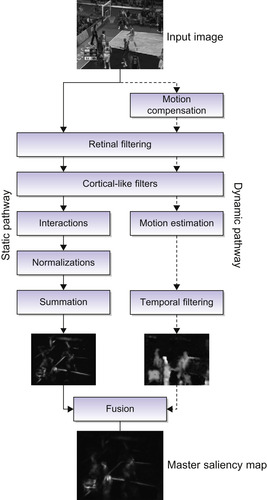 |
| Figure 30.1
The bottom-up visual saliency model.
|
The retinal model is primarily based on the primate's retina, which imitates the photoreceptor, horizontal, bipolar, and ganglion cells. It takes an input visual scene, and decomposes it into two types of information: the parvocellular output that enforces equalization of the visual by increasing its contrast. Next in the order, the magnocellular that responds to higher temporal and lower spatial frequencies. Analogous to a primate's retina, the ganglion cells respond to high contrast, whereas the parvocellular output highlights the borders among the homogeneous regions, thus exposing more detail in the visual input.
The primary visual cortex is a model of simple cell receptive fields that are sensitive to visual signal orientations and spatial frequencies. This can be imitated using a bank of Gabor filters organized in two dimensions, which is closely related to the processes in the primary visual cortex. The retinal output is convolved to these Gabor filters in the frequency domain.
In the primate's visual system, the response of a cell is dependent on its neuronal environment, that is, its lateral connections. Therefore, this activity can be modeled as a linear combination of simple cells interacting with their neighbors. This interaction may be inhibitory or excitory, depending on the orientation or the frequency: excitory when in the same direction; otherwise, it is inhibitory. The energy maps from the visual cortical filters and interaction phase are normalized. This model uses a technique
[6]
proposed by Itti for strengthening the intermediate results.
Ultimately, a saliency map for the static pathway is extracted for the input visual, simply by summing up all the energy maps. It is significant that the resulting map has salient regions, that is, those with the highest energies, which can be observed in
Figure 30.2
by energy located on such objects.
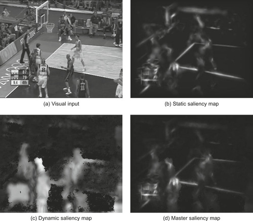 |
| Figure 30.2
Results of the visual saliency model.
|
30.2.2. Dynamic Pathway
On the other hand, the dynamic pathway finds salient regions in a moving scene. The dynamic pathway uses camera motion compensation
[8]
for compensation of dominant motion against its background. This compensation is followed by retinal filtering to illuminate the salient regions before motion estimation.
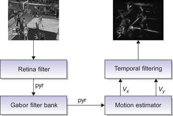
After the preprocessing, two-dimensional estimation
[2]
is used to find local motion with respect to the background. The algorithm is based on Gabor filters to decompose the image into its sub-bands. These equations are then used to estimate the optical flow between two images. After Gabor filtering, we calculate a system of N equations for each pixel at each time t using spatial and temporal gradients to get an overconstrained system. To resolve this system, which is fairly noisy, we use the method of iterated weighted least squares within the motion estimator. In the end, temporal filtering is performed on the sequence of images, often used to remove extraneous information. Finally, we get the dynamic saliency map.
30.2.3. Fusion
The saliency maps from both the static and dynamic pathways exhibit different characteristics; for example, the first map has larger salient regions based on textures, whereas the other map has smaller regions, depending on the moving objects. Based on these features, the maps are modulated using maximum and skewness, respectively, and fused together to get a final saliency map.
Often visual saliency models incorporate a number of complex tasks that make a real-time solution quite difficult to achieve. This objective is only achievable by simplification of the overall model as done by Itti
[5]
and Ouerhani
[9]
. Consequently, including other processes into the existing model is impossible. Over the years, GPUs have evolved from fixed-function architecture into completely programmable shader architecture. All together with a mature programming model like CUDA
[1]
makes the GPU platform a preferable choice for acquiring high-performance gains. Generally, vision algorithms are a sequence of filters that are relatively easier to implement on the GPU's massively data-parallel architecture. The graphics device is also cheaper and easier to program than its counterparts. In addition, the graphics device is accessible to everyone.
To start with the mapping of the
Algorithm 1
onto GPU, it is partitioned into data-parallel portions of code that are isolated into separate kernels. Then, the input data is transferred and stored on the device memory, which afterward is used by the kernels. After all the memory declarations on the device, the host sequentially initiates all the data-parallel kernels. First, some preprocessing using a retinal filter and Hanning mask is done that gives more detail to the visual input. Second, this data in the frequency domain is treated with a 2-D Gabor filter bank using six orientations and four frequency bands, resulting in 24 partial maps. Third, the pathway is moved back to the spatial domain before interactions among these maps. These interactions inhibit or excite the data values, depending on the orientation and frequency band of a partial map. Fourth, the resulting values are normalized between a dynamic range before applying Itti's method for normalization, and suppressing values lower than a certain threshold. Finally, all the partial maps are accumulated into a single map that is the saliency map from the static pathway.

30.3.2. The Dynamic Pathway
Similar to the implementation of the static pathway, we first perform task distribution of the algorithm and realize its sequential version. Some of the functional units are recursive Gaussian filter, Gabor filter bank to break the image into sub-bands of different orientations, Biweight Tuckey motion estimator, Gaussian prefiltering for pyramids, spatial and temporal gradient maps for estimation, and bilinear interpolation. After testing these functions separately, we put them together to give a complete sequential code. The algorithm being intrinsically parallel allows it to be easily ported to CUDA.
Algorithm 2
describes the dynamic pathway, where first camera motion compensation and retinal filtering are done as a preprocessing on the visual input. Afterward, the preprocessed input is passed on to the motion estimator implemented using third-order Gabor filter banks. The resulting motion vectors are normalized using temporal information to get a dynamic saliency map.
The saliency maps from both the static and dynamic pathways are copied back onto the host CPU, where they are fused together outputting a saliency map. The two saliency maps from different
pathways and the final output saliency map are shown in
Figure 30.2
. Moreover,
Figure 30.3
illustrates the block diagram of the GPU implementation of the visual saliency model.
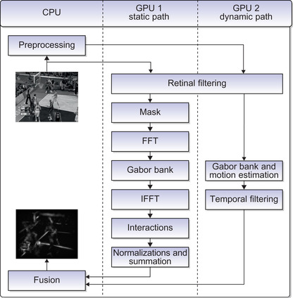 |
| Figure 30.3
GPU implementation of the visual saliency model.
|
Importance of Optimizations
One of the biggest challenges in optimizing GPU code for data-dominated applications is the management of the memory accesses, which is a key performance bottleneck. Memory latency can be several hundreds, or even thousands, of clock cycles. This can be improved first by memory coalescing when memory accesses of different threads are consecutive in memory addresses. This process allows the
global memory controllers to execute burst memory accesses. The second optimization is to avoid such memory accesses through the use of a cache memory, internal shared memories, or registers. Most important, shared memory is an on-chip high-bandwidth memory shared among all the threads on a single SM. It has several uses: as a register extension, to avoid global memory accesses, to give fast communication among threads, and as a data cache.
30.3.3. Various CUDA Kernels
The static pathway includes the retina filter with low-pass filters using 2-D convolutions, the normalizations with reduction operations, simple shifts operations, and fourier transforms. On the other hand, the dynamic pathway involves recursive guassian filters, projection, modulation/demodulation, and kernels for calculation of spatial and temporal gradients that are simple and classically implemented. Notabaly, the kernels that are compute intensive and interesting to be implemented on the GPU are the interactions kernel and Gabor filter bank from the static pathway, as well as the motion estimator kernel from the dynamic pathway. Hence, we present these kernels because they can be potentially improved by employing various optimizations and making several adjustments to the kernel launch configurations.
Interactions Kernel
In the primate's visual system, the response of a cell is dependent on its neuronal environment, that is, its lateral connections. This activity can be modeled as a linear combination of simple cells interacting with their neighbors.
 The resulting partial maps
E
int
after taking into account interactions among different orientation maps
E
from the Gabor filter bank are the visual input's energy as a function of spatial frequency
f
and orientation
θ
.
The resulting partial maps
E
int
after taking into account interactions among different orientation maps
E
from the Gabor filter bank are the visual input's energy as a function of spatial frequency
f
and orientation
θ
.
The block diagram in
Figure 30.4
shows the simple interactions kernel for 32 complex numbers for 32 partial maps from the Gabor filter bank that are first accessed from the global memory in a coalesced manner and placed in shared memory
“maps”
in separate regions for real and complex portions of the number. These numbers are then accessed in a random manner and converted into 16 real numbers. These results are stored in the
“buf”
shared memory variable, which is afterward used as prefetched data for the next phase of neuronal interactions.
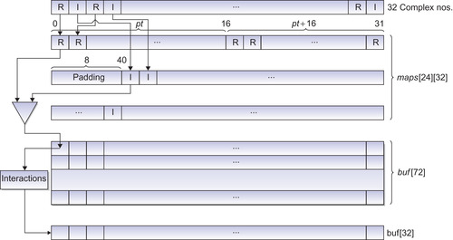 |
| Figure 30.4
A block diagram of a data-parallel interaction kernel.
|
We'll now discuss coalescing using shared memory. A method to avoid noncoalesced memory accesses is by reordering the data in shared memory. To demonstrate the uses of shared memory, we take an example kernel, as shown in
Listing 30.1
, which is illustrated using a block diagram shown in
Figure 30.4
. Here, the data values are in a complex format consisting of two floats. The very first step is fetching the values into shared memory, where each float is read by a separate thread as shown in line 12 in
Listing 30.1
. These global memory accesses are coalesced, as contiguous floats are read shown in line 24 in
Listing 30.1
. Furthermore, we use two shared buffers, one for real part, and the other for imaginary part. This arrangement provides uncoalesced shared memory accesses during computation in lines 30 and 31 in
Listing 30.1
to convert the complex numbers into real and also to scale down the
output from the unnormalized Fourier transforms done using the CUFFT library.
Table 30.1
shows the performance gains after coalescing global memory accesses.
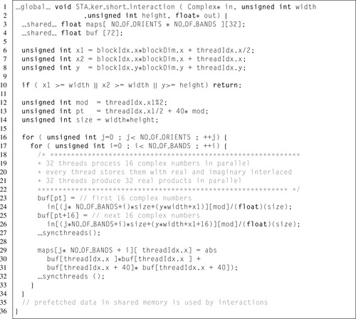
Multiple threads accessing the same bank may cause conflicts. In the case of shared memory bank conflicts, these conflicting accesses are required to be serialized either using an explicit stride based on the thread's ID or by allocating more shared memory. In our case, when the thread's ID is used to access shared memory, a conflict occurs, as thread 0 and thread 1 access the same bank. Thus, we use a stride of 8 to avoid any conflicts, as shown in line 13 in
Listing 30.1
. Although a multiprocessor takes only 4 clock cycles doing a shared memory transaction for an entire half warp, bank conflicts in the shared memory can degrade the overall performance, as shown in
Table 30.2
.
| GPU time | Occupancy | Warp serialize | |
|---|---|---|---|
| With bank conflicts | 8.13 ms | 0.125 | 75,529 |
| Without bank conflicts | 7.9 ms | 0.125 | 0 |
Another use of shared memory is to prefetch data from global memory and cache it. In the example kernel, the data after conversion and rescaling are cached, as shown in line 29 in
Listing 30.1
. and this prefetched data is used in the next phase of interactions.
30.3.4. Motion Estimator Kernel
The motion estimator
[2]
presented here employs a differential method using Gabor filters to estimate local motion. The estimated speeds are obtained by solving a robust system of equations of optical flow. It works on the principle of conservation of brightness; that is, the luminance of any pixel remains the same for a certain interval of time. Consider that
I
(x
,
y
,
t
) represents the brightness function for the sequence of images, and then according to the hypothesis of conversation of total luminance, its time
derivative is zero. Therefore, the motion vector
υ
(p
) = (υ
x
,
υ
y
) can be found using the equation of optical flow:
 where ▽
I
(x
,
y
,
t
) is the spatial gradient of luminance
I
(x
,
y
,
t
). Using this equation, we get a velocity component parallel to this spatial gradient. The information from the spatial gradients in different directions can be used to find the actual movement of an object. If the intensity gradient is ▽
I
= 0, then the motion is negligible, whereas motion in one direction represents the edges.
where ▽
I
(x
,
y
,
t
) is the spatial gradient of luminance
I
(x
,
y
,
t
). Using this equation, we get a velocity component parallel to this spatial gradient. The information from the spatial gradients in different directions can be used to find the actual movement of an object. If the intensity gradient is ▽
I
= 0, then the motion is negligible, whereas motion in one direction represents the edges.
To perform a proper estimation of motion, we average the movement corresponding to its spatial neighborhood. This spatial neighborhood is required to be large enough to avoid any ambiguous resulting motion vectors. Thus, to get a spatial continuity within the optical flow, we convolve the spatio-temporal image sequence with a Gabor filter bank:
 The bank consists of
N
filters
G
i
with the same radial frequency. The result is a system of N equations for each pixel with a velocity vector composed of two components (υ
x
,
υ
y
). This system of equations can be represented as:
The bank consists of
N
filters
G
i
with the same radial frequency. The result is a system of N equations for each pixel with a velocity vector composed of two components (υ
x
,
υ
y
). This system of equations can be represented as:
 This overdetermined system of equations is solved by using the method of least squares (Biweight Tuckey test)
[2]
.
This overdetermined system of equations is solved by using the method of least squares (Biweight Tuckey test)
[2]
.
The estimator uses multiresolution patterns to allow robust motion estimation over a wide range of speeds. Here, the image is subsampled into multiple scales resulting in a pyramid, where the approximation begins with the subsampled version of the image at the highest level. This process is iterated until applied to the image with original resolution. This multiscale approach is equivalent to applying a Gabor bank of several rings with different scales. The final result for the estimator is a motion vector for each pixel.
In the motion estimator prefetch kernel, we use spatial and temporal gradient values to get
N
(2
N
− 1) solutions that are used to perform iterative weighted least-square estimations. These numerous intermediate values are stored as array variables because the register count is already high. Unfortunately, this process leads to costly global memory accesses that can be avoided by placing some
values in shared memory as shown in line 7 in
Listing 30.4
. Consequently, we get a solution with the lesser memory accesses and efficient use of limited resources on the device. We achieved performance gains by carefully selecting the amount of shared memory without compromising the optimal number of active blocks residing on each SM.
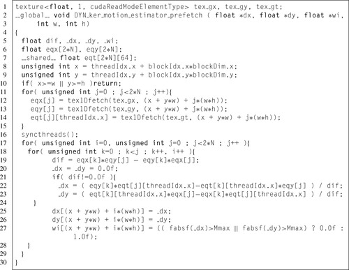 |
| Listing 30.4. |
| The prefetch motion estimator kernal.
|
In the motion estimator kernel illustrated in
Listing 30.2
, there is a limitation of higher register count owing to the complexity of the algorithm; hence, using the motion estimator kernel results in a reduced number of active thread blocks per SM. In our naive solution, the register count is 22, and this number can be considerably reduced to 15 registers per thread block using shared memory for some local variables as done in line 6 of
Listing 30.2
. Consequently, the occupancy increased from 0.33
to 0.67 with eight active thread blocks residing on each SM. These variables to be placed in shared memory are carefully selected to reduce the number of synchronization barriers needed.
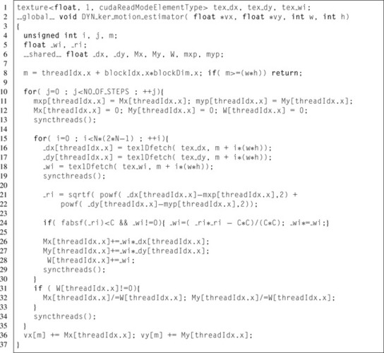 |
| Listing 30.2. |
| The motion estimator kernel.
|
Texture memory provides an alternative path to device memory, which is faster. This is because of specialized on-chip texture units with internal memory to allow buffering of data from device memory. It can be very useful to reduce the penalty incurred for nearly coalesced accesses.
In our implementation, the main motion estimation kernel exhibits a pattern that requires the data to be loaded from device memory multiple times; that is, we calculate an
N
(2
N
− 1) system of equations for 2*N levels of spatial and temporal gradients. Because of memory limitations of the device, it is not feasible to keep the intermediate values. Therefore, we calculate these values at every pass of the estimator leading to performance degradation because of higher device memory latency. As a solution, the estimation kernel can be divided into two parts: one calculates the system of equations, while the other uses these equations for estimation through texture memory. Here, texture memory's caching mechanism is employed to prefetch the data calculated in the prefetch kernel shown in
Listing 30.3
, thereby reducing global memory latency and yielding up to a 10% performance improvement. The profile of the gains due to various optimizations is illustrated in
Table 30.3
.
| Listing 30.3. |
| Using shared memory to reduce global memory accesses.
|
30.3.5. Gabor Kernel
Cortical-like filters are a model of simple cell receptive fields that are sensitive to visual signal orientations and spatial frequencies. This can be imitated using a bank of Gabor filters organized in two dimensions; that is, closely related to the processes in the primary visual cortex. A Gabor function is defined as:
The retinal output is filtered using Gabor filters implemented in the frequency domain after applying a mask. The mask is similar to a Hanning function to produce non-uniform illumination approaching zero at the edges. The visual information is processed in different frequencies and orientations in the primary cortex; that is, the model uses six orientations and four frequencies to obtain 24 partial maps as shown in
Figure 30.5
. These filters demonstrate optimal localization properties and a good compromise of resolution between frequency and spatial domains. Finally, the
Listing 30.5
illustrates the kernel of the Gabor filters using constant and texture memories.
 |
| Figure 30.5
Gabor filter bank configuration.
|
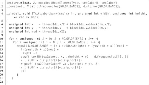 |
| Listing 30.5. |
| A Gabor bank filtering kernel producing 24 partial maps.
|
30.3.6. Multi-GPU Implementation
Multi-GPU implementation is quite interesting to increase the computational efficiency of the entire visual saliency model. We have employed a shared-system GPU model, where multiple GPUs are installed on a single CPU. If the devices need to communicate, they do it through the CPU with no
inter-GPU communication. A CPU thread is created to invoke kernel execution on a GPU; accordingly, we will have a CPU thread for each GPU. To successfully execute our single GPU solution on multi-GPUs, the parallel version must be deterministic. Our first implementation, the two pathways of the visual saliency model — static and dynamic — are completely separate with no inter-GPU communication required. The resultant saliency maps are simply copied back to the host, where they can be fused together into the final saliency map.
Pipeline Model
In this multi-GPU implementation, we employ a simple domain decomposition technique by assigning separate portions of the task to different threads. As soon as any thread finds an available device, it fetches the input image from the RAM to device memory and invokes the execution of the kernel. The threads wait until the execution of the kernel is complete and then gather their respective results back.
In our implementation as illustrated in
Figure 30.6
, we have three threads that are assigned different portions of the visual saliency model. For instance, thread 0 calculates the static saliency map; thread 1 does the retinal filtering and applies the Gabor filters bank; and thread 2 performs the motion estimation
outputting the dynamic saliency map to the host. The division of the dynamic pathway is done based on computational times of different kernels; we find that the suitable cut will be after recursive Gaussian filters that are followed by the motion estimator, as shown in
Figure 30.7
. Each half of this cut takes ∼60 ms, which is half of 130 ms for the entire pathway. The inter-GPU communication between thread 1 and thread 2 involves the transfer of the N-level pyramid for the input image treated with the retinal filter and Gabor bank. Afterward, thread 2 is responsible for the estimation. Finally, the static and dynamic saliency maps from thread 0 and thread 2 are fused into the final visual saliency map. Consequently, using a pipeline cuts off the time to calculate the entire model to ∼50 ms instead of 150 ms for the simple solution.
 |
| Figure 30.6
A block diagram of the multi-GPU pipeline model.
|
 |
| Figure 30.7
A block diagram of the decompose dynamic pathway.
|
In such a multithreaded model, there is complexity involved in selecting an efficient strategy for creation and destruction of threads, resource utilization, and load balancing. Also, inter-GPU communication between GPUs might be an overhead affecting the overall performance. This overhead can be tackled by overlapping communications with computations using streaming available in the CUDA programming model.
30.4. Results
All implementations were tested on a 2.80 GHz system with 1 GB of main memory, and Windows 7 running on it. On the other hand, the parallel version was implemented using the latest CUDA v3.0 programming environment on NVIDIA GTX285 series graphics cards.
30.4.1. Speedup of Static Pathway
In the algorithm, a saliency map is produced at the end of the static pathway, which identifies the salient regions in the visual input. These stages include a Hanning mask, Retinal filter, Gabor filter
bank, interaction, normalization, and fusion. All these stages show a great potential to be parallelized and are isolated within separate kernels. Initially, the model is implemented using MATLAB that happens to be extremely slow because it involves a number of compute-intensive operations; for example, 2-D convolutions, conversions between frequency and spatial domains, and Gabor banks producing 24 partial maps that are further processed. As a result, a single image would take about 18 s to pass through the entire pathway in our MATLAB code, making it unfeasible for real-time applications. The target of the second implementation in C is to identify the data-parallel portions after writing it in a familiar language. It includes many optimizations and also the use of a highly optimized FFTW library for Fourier transforms, but the speedup witnessed is only 2.17x.
At first, the porting of the data-parallel portions into separate kernels for the GPU can be simple. But the code requires many tweaks to achieve the promised speedup, and tweaking the code happens to be the most complex maneuver. Although the very first implementation involved partitioning into data-parallel portions, which resulted in a speedup of about 396x, the peak performance topped over to 440x after we made various optimizations.
Table 30.5
shows timings for the different kernels, while performance gains after optimizations are presented in
Table 30.4
. To test the performance of this pathway, we use an image size of 640 × 480 pixels.
30.4.2. Speedup of Dynamic Pathway
To evaluate the performance gains of the dynamic pathway, we compare the timings on the GPU against the sequential C and MATLAB code, as shown in
Table 30.6
.
Table 30.7
shows times for the various kernels in the pathway. We used three datasets of images “Treetran,” “Treediv,” and “Yosemite” for comparison, the first two with resolution of 150 × 150 pixels, while 316 × 252 pixels for the last one.
| Treetran | Treediv | Yosemite | |
|---|---|---|---|
| MATLAB | 13.30 s | 12.86 s | 46.61 s |
| C | 1.75 s | 1.76 s | 6.28 s |
| CUDA | 0.12 s | 0.12 s | 0.30 s |
30.4.3. Precision
The vision algorithm implemented in CUDA is ported from MATLAB code, where all the computations are done entirely in double precision; fortunately, the effects of low precision in parallel implementation are not obvious. The main reason is the type of algorithm, that is, whether it can produce acceptable results, or ones that are usable. Here, the resultant saliency map may be inaccurate, but visually fine
with a universal image quality index
[12]
of 99.66% and two digit precision among the 24 bits of a float mantissa.
Figure 30.8
shows the mean error with respect to the reference during different stages of the pathway. We observe that the accuracy increases along the progressing stages because of the reduction of information, more evident during Gabor filtering and normalization phases until finally ending up in regions that are salient.
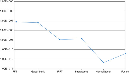 |
| Figure 30.8
The effect of lower-precision support on the result.
|
30.4.4. Evaluation of Results
To evaluate the correctness of the motion estimator, we calculate the error between estimated and real optical flows using the equation below:
 where
a
e
is the angular error for a given pixel with (u
,
v
) the estimated and (u
r
,
v
r
the real motion vectors. We used “treetran” and “treediv” image sequences for the evaluation, showing translational and divergent motion, respectively
[2]
. The results shown in
Table 30.8
are obtained using “treetran” and “treediv” image sequences of sizes 150 × 150 pixels.
where
a
e
is the angular error for a given pixel with (u
,
v
) the estimated and (u
r
,
v
r
the real motion vectors. We used “treetran” and “treediv” image sequences for the evaluation, showing translational and divergent motion, respectively
[2]
. The results shown in
Table 30.8
are obtained using “treetran” and “treediv” image sequences of sizes 150 × 150 pixels.
The results of the visual saliency model can be evaluated using Normalized Scanpath Saliency (NSS)
[10]
as shown in
Table 30.9
. This criteria compares the eye fixations of the subjects with the salient areas in the resulting saliency map. The NSS metric corresponds to a Z-score that expresses the divergence of experimental results (eye fixations) compared with model mean as a number of standard deviations of the model. The higher value of the Z-score suggests a correspondence between the eye fixations and locations calculated by the model. We calculate the NSS with the equation:
 where
M
h
(x
,
y
,
k
) is the human eye position density map normalized to unit mean, and
M
m
(x
,
y
,
k
) is a model saliency map. The value of NSS is zero if there is no correspondence between eye positions and salient regions. Whereas, if positive then strong correspondence, and the rest show anti-correspondence.
where
M
h
(x
,
y
,
k
) is the human eye position density map normalized to unit mean, and
M
m
(x
,
y
,
k
) is a model saliency map. The value of NSS is zero if there is no correspondence between eye positions and salient regions. Whereas, if positive then strong correspondence, and the rest show anti-correspondence.
30.4.6. Real-Time Streaming Solution
OpenVIDIA
[4]
is an open source platform that provides an interface for video input, display, and programming on the GPU that is facilitated with a bunch of high-level implementations of a number of image-processing and computer vision algorithms using OpenGL, Cg, and CUDA. These implementations include feature detection and tracking, skin tone tracking, and projective panoramas.
After the parallel implementation of the visual saliency algorithm, we used OpenVIDIA to demonstrate the real-time processing. The demonstration is done on a quad-core machine with three GPUs installed, and the library is used to interface with the webcam. This resulted in execution of the static
pathway at 28 fps on the platform shown in
Figure 30.9
. Finally, the performance gains on GPU will enable our model to be used for various applications such as the automatic video reframing process
[3]
. This application extracts a cropping window using the regions of interest from the model. These windows are then smooth to increase the viewing experience.
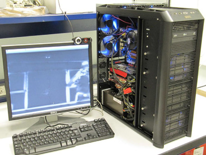 |
| Figure 30.9
A platform for a real-time solution.
|
30.5. Conclusion
In this chapter, we presented the multi-GPU implementation of a visual saliency model to identify the areas of attention. The main advantage of the performance gain accomplished will allow the inclusion of face recognition, stereo, audio, and other complex processes. Consequently, this real-time solution finds a wide application for several research and industrial problems, such as video compression, video reframing, frame quality assessment, visual telepresence and surveillance, automatic target detection, robotics control, super-resolution, and computer graphics rendering.
References
[1]
NVIDIA Corporation: NVIDIA CUDA compute unified device architecture programming guide v3.0. NVIDIA Corporation.
http://developer.nvidia.com/cuda
(accessed 12.31.10).
[2]
E. Bruno, D. Tarjan,
Robust motion estimation using spatial gabor-like filters
,
Signal Process
82
(2002
)
297
–
309
.
[3]
C. Chamaret, O. Le Meur,
Attention-based video reframing: validation using eye-tracking
,
In:
Pattern Recognition, 2008
ICPR 2008. 19th International Conference on, IEEE, Tampa, FL
. (December 2008
), pp.
1
–
4
.
[4]
J. Fung, S. Mann, C. Aimone,
Openvidia: parallel gpu computer vision
,
In:
MULTIMEDIA ’05: Proceedings of the 13th Annual ACM International Conference on Multimedia
(2005
)
ACM
,
New York
, pp.
849
–
852
.
[5]
L. Itti,
Real-time high-performance attention focusing in outdoors color video streams
,
In: (Editors: B. Rogowitz, T.N. Pappas)
Proceedings of SPIE Human Vision and Electronic Imaging VII, HVEI ’02
(2002
)
SPIE Press
,
San Jose
, pp.
235
–
243
.
[6]
L. Itti, C. Koch, E. Niebur,
A model of saliency-based visual attention for rapid scene analysis
,
IEEE Trans. Pattern Anal. Mach. Intell.
20
(1998
)
1254
–
1259
.
[7]
S. Marat, T. Ho Phuoc, L. Granjon, N. Guyader, D. Pellerin, A. Guérin-Dugué,
Modelling spatio-temporal saliency to predict gaze direction for short videos
,
Int. J. Comput. Vision
82
(2009
)
231
–
243
.
[8]
J.M. Odobez, P. Bouthemy,
Robust multiresolution estimation of parametric motion models applied to complex scenes
,
J. Vis. Commun. Image Represent
6
(1994
)
348
–
365
.
[9]
N. Ouerhani, H. Hgli,
Real-time visual attention on a massively parallel simd architecture
,
Real-Time Imaging
9
(2003
)
189
–
196
.
[10]
R.J. Peters, A. Iyer, L. Itti, C. Koch,
Components of bottom-up gaze allocation in natural images
,
Vision Res.
45
(2005
)
2397
–
2416
.
[11]
A computational saliency model integrating saccade programming
,
In: (Editors: T. Ho-Phuoc, A. Guérin-Dugué, N. Guyader, P. Encarnação, A. Veloso)
BIOSIGNALS
(2009
)
INSTICC Press
, pp.
57
–
64
.
[12]
Z. Wang, A.C. Bovik,
A universal image quality index
,
IEEE Signal Process. Lett.
9
(2002
)
81
–
84
.
..................Content has been hidden....................
You can't read the all page of ebook, please click here login for view all page.