
Chapter 33. Haar Classifiers for Object Detection with CUDA
Anton Obukhov
This gem covers aspects of the approach to object detection proposed by Viola and Jones
[1]
. The algorithm is discussed along with its well-known implementation from the OpenCV library. We describe the creation process of the GPU-resident object detection pipeline step by step and provide analysis of intermediate results and the pseudo code. Finally, we evaluate the CUDA implementation and discuss its properties.
The gem is targeted at the users and programmers of computer vision algorithms. The implementation and analysis sections require basic knowledge of C/C++ programming languages and CUDA architecture.
33.1. Introduction
Object detection in still images and video is among the most-demanded techniques that originate from computer vision. Paul Viola and Michael Jones came up with their framework for object detection in early 2001
[1]
and since that time, the framework has not changed significantly. It is widely used in a variety of software and hardware applications that incorporate elements of computer vision, like the face detection module in video conferencing, human-computer interaction, and digital photo cameras.
Although the original framework provides several optimizations that allow rejection of the greater part of potential workload on early stages of processing, the algorithm is still considered to be computationally expensive. At the dawn of high-definition imaging sensors and hybrid CPU-GPU architectures, the problem of performing fast and accurate object detection becomes especially important.
33.2. Viola-Jones Object Detection Retrospective
The core algorithm of object detection, as described in
[1]
, consists of two steps:
• Creation of the object classifier
• Application of this classifier to an image
Hereby, an
object classifier
is a function applied to a region of pixels. The function evaluates to 1 in case the region is likely to be a representation of the object, and to 0 otherwise.
Throughout the chapter, the term “
object
” will stand for
a constrained view of any tangible object of some predefined structure, material, and shape
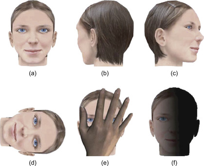
. Such elaborate definition comes as a constraint of the mathematical model, serving as the basis for the object detection algorithm. In this context, a “human head” is not an object because several views of a human head exist that differ in structure from each other: the front view, the profile view, the view from the back (Figure 33.1
), and so on. The “frontal face view” is much closer to the correct definition, but it still needs specification of the view constraints, like sufficient lighting conditions and horizontal alignment. As for the structure, material, and shape, the counterexamples of the previous definition are demonstrated in
Figure 33.2
.
 |
| Figure 33.1
(a) A properly aligned fully visible frontal face. (b), (c) Unconstrained viewpoint. (d) Unconstrained alignment. (e) Unconstrained occlusion conditions. (f) Unconstrained lighting conditions.
|
 |
| Figure 33.2
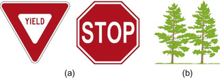
(a) Varying shape. (b) Undefined structure.
|
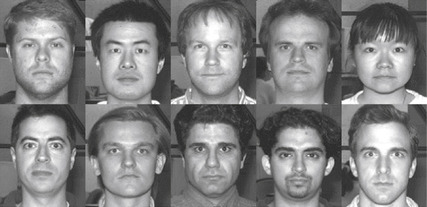
In order to accomplish the training step and create an object classifier, one needs to collect a training set of images that contain depiction of the object of interest (Figure 33.3
) and images containing
anything else. The typical size of such a training set can start from several thousand images. The process of object classifier creation is very computationally expensive: a training program loads all images into the memory and performs a thorough search of similarities between images of the object. The training process needs to be done only once, and its output is a compact representation of the data, that according to the training model represents a set of formal rules for distinguishing between an image of the object of interest and any other image. This data is the object classifier itself.
 |
| Figure 33.3
Example of the face detector training database entries (from the Yale Face Database B).
|
In the original work, Viola and Jones trained the frontal face classifier for images of 24 × 24 pixels size. Such a small size of the test region appears to be optimum for the task of face detection because it contains a reasonable amount of details and at the same time keeps training time to about a week using a modern workstation PC.
Later, Rainer Lienhart created his own set of frontal face classifiers for the Open Source Computer Vision library (OpenCV), which were trained to classify regions of 20 × 20 pixels size. Those classifiers are stored as XML files of an average size of 1 MB. With the wide adoption of OpenCV in open source and commercial products, Lienhart's classifiers have become a de facto standard for general-purpose frontal face detection. They are well studied and usually meet requirements for a face detection system. In case the requirements are not met (for instance, if a user wants to create a classifier for some other object like faces in profile), OpenCV provides the training framework for the new classifier creation.
Although there is a certain interest in increasing the speed of classifier creation (for instance, for semiautomatic video annotation and tagging), this gem concentrates on the second step of the object detection task — the object classifier application. OpenCV and the Lienhart frontal face classifier will be used as references for the implementation using NVIDIA CUDA technology.
33.2.1. The Core Algorithm
Now, when a user has an object classifier trained on images of size
M
×
N
and an input image of much higher dimensions, it is possible to detect all instances of the object of interest in the image. This is achieved by applying the classifier to every region of pixels of size
M
×
N
on a large set of scales of the input image (Figure 33.4a
). OpenCV implements this algorithm in the
CascadeClassifier::detectMultiScale
function, which also takes the image buffer, scale step,
a few options, and the pointer to the output list to store the detections. Because application of the object classifier to a region of pixels doesn't depend on anything but the input pixels, all classifier applications can be performed in parallel. OpenCV takes this opportunity in case it was compiled with Intel Threading Building Blocks support enabled.
 |
| Figure 33.4
(a) Multiple detections at various scales. (b) Filtered hypothesis.
|
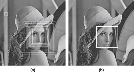
Usually a classifier finds many matches around the scope of the real object location (Figure 33.4a
). This happens as a result of the insensitivity of the object classifier to tiny shifts, rotations, and scaling of the object of interest. This phenomenon is closely related to the generalization property of the object classifier — the ability to deal successfully with images of the same object that didn't participate in the training set. To get one final hypothesis per actual object representation, the detections have to be partitioned into equivalence classes and filtered. The partitioning is performed using the criterion of rectangular similarity, that is, if the area of intersection relative to their sizes is greater than some predefined threshold.
Figure 33.4a
contains two obvious classes: one in the top left corner, which comes from the detector's false-positive detections, and one close to the actual face location. The filtration of the detections classes is performed according to two simple rules:
• If the class contains a small amount of detections, then it is believed to be a false positive and is dropped.
• The rest of the classes are averaged, and the final hypotheses are presented as face detections (Figure 33.4b
).
As can be seen, there are a lot of independent operations on the regions, telling target objects apart from nonobjects. But still the overall amount of computations is overwhelming. In order to speed up processing, Viola and Jones proposed the
cascade
scheme of the object classifier function. As shown in
Figure 33.5
, the idea is to represent an object classifier in a series of smaller object classifiers in order to reject nonobjects as fast as possible. To be detected by the cascade, an object has to pass all stages of the object classifier cascade. Such an early-termination processing scheme drastically reduces the overall workload.
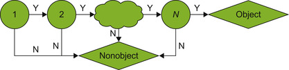 |
| Figure 33.5
Strong classifiers cascade.
|
As stated in
[4]
, the frontal face classifier cascade of 20 stages is trained to reject 50% of non-faces on every stage. At the same time every stage falsely eliminates 0.1% of true face patterns. The integrate characteristics of such a cascade are given in
Table 33.1
.
33.2.2. Object Classifier Cascade Structure
The classifier cascade (Figure 33.5
) consists of a chain of stages, also known as
Strong Classifiers
(in
[1]
) and the
“Committees” of Classifiers
(in
[4]
). Although these names were given to emphasize the complex structure of the entity, throughout the gem a stage will be referred to as simply the
classifier
. A classifier is capable of acting as an object classifier on its own account, and this had been a common approach before Viola and Jones proposed the cascade scheme. Having a solid object classifier represented by one classifier has the following disadvantages:
• It is much harder to train the monolithic classifier with acceptable detection rates compared with the cascade of classifiers with the same properties.
• There is no early termination when testing unlikely object-containing regions.
The OpenCV classifier (H
) structure is presented in
Figure 33.6
. It encapsulates a set of
K
weak classifiers
(h
i
) and the stage threshold (T
). A weak classifier got its name because it is not capable of classifying regions on the object level; all it does is calculate some function on the region of pixels and produce the binary response. For the sake of computation simplicity, the function was chosen to be based on Haar wavelets (features). The formula in
Table 33.2
(left) contains the equation of the strong classifier (X
denotes the region of pixels of the
M
×
N
size being tested).
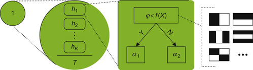 |
| Figure 33.6
Left to right: the stage of the classifier cascade, the classifier, the weak classifier, and various Haar features.
|
As for the weak classifier, in the simplest case it consists of the threshold
φ
i
and one
Haar feature
f
i
. A feature in the weak classifier is essentially a rectangular template, which is laid over the tested region in a specific location. The black-and-white coloring scheme of the template indicates the change of a sign when taking the sum of underlying pixel values of the input image: black pixels make a positive contribution, while white corresponds to a negative contribution. This summation evaluates
f
i
(X
), which is then compared with the threshold. The classifier that consists of such binary weak classifiers is called “stump-based.” The formula in
Table 33.2
(right) contains the equation of the weak classifier.
The OpenCV implementation of Haar features consists of a list of tuples (rectangle, weight). The rectangle corners coordinates are integers and must lie inside of the classifier
M
×
N
window. After summing the pixels under the rectangle, the sum is multiplied by the weight, which is represented by a floating-point value.
Generally, a weak classifier can be represented as a decision tree, where each node contains a Haar feature and the corresponding threshold, and leaves contain
α
values. Evaluation of such a weak classifier takes
D
times more time than a stump-based weak classifier, where
D
is the depth of the decision tree. An example of such a weak classifier is shown in
Figure 33.7
.
 |
| Figure 33.7
An example of a tree-based weak classifier.
|
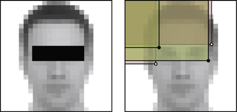
The illustration in
Figure 33.8
helps to understand Haar features better. The two features are taken from the first stage of Lienhart's cascade for face detection; they are put over the 20 × 20 region, which actually contains a man's face. The first required feature can be described as the assumption that an image of the human face has a bright area on the forehead and a dark area on the eyes (due to shadowing, eyebrows, eyelashes, and iris). The second feature makes a similar assumption about the nose bridge area, which is always brighter than the eyes due to high local skin reflection properties. Of course, these two rules of thumb don't suffice to claim that the region is actually a face. According to
[2]
, if provided with enough weak classifiers, each acting slightly better than random, one can train a strong classifier with as low a training error rate as one wishes. According to
[1]
, the classifier of two presented features rejects over half of “non-faces” and passes ∼100% “faces” to the next stages of the classifier cascade.
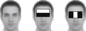 |
| Figure 33.8
Haar features from the first stage classifier of the face detection cascade.
|
In order to calculate the response of a weak classifier in a straightforward way, one would need to sum all values of pixels under the white part of the feature template and then calculate the same sum for the black part of the template and subtract the sums. For a feature of 10 × 10 pixels and the initial scale
S
= 1 this would require 100 memory accesses and 100 additions/subtractions. On the scale
S
= 4, the 10 × 10 feature will map to a region of 40 × 40 pixels, and its calculation will cost 1600 memory accesses and the same amount of additions/subtractions. The
integral image
representation was introduced to fight the complexity when calculating features on any scales. An input image (F
) is converted to an integral image (I
) using the first formula from
Table 33.3
.
 |
As can be noted from the formula, the integral image representation is 1 pixel wider and higher than the original image. Each pixel of the integral image contains the sum of all pixels of the input image to the left and top of the location. Using this representation, any rectangular area of pixels can easily be summed with only four memory accesses and three additions/subtractions, as shown in the second formula in
Table 33.3
. For example, to calculate the sum of pixels under the eye rectangle (Figure 33.9
), one needs to take the sum of pixels of both dark rectangles (with the solid black circle in the bottom-right corner) and subtract the sum of pixels of both light rectangles (which has the black-and-white circle). Here all four rectangles have their top-left corner in the image origin, and rectangular sums can be obtained from the integral image.
 |
| Figure 33.9
Visualization of rectangular area pixels sum calculation with the integral image. Integral image values at solid black circle positions give positive contribution, the values at black-and-white circles should be subtracted.
|
To minimize the effect of varying lighting conditions, the original classifier cascade described in
[1]
was trained on variance-normalized images. A
variance-normalized image
can be obtained by dividing image pixels by the standard deviation of all pixels. The value can be easily calculated from the image pixels using the last formula from
Table 33.4
.

Variance calculation can also benefit from integral images, but it requires one more representation — the
squared integral image
, which represents the integral image of all pixel values squared. To calculate a variance of a pixels region using the formula shown in
Table 33.4
, one would calculate the mean using the integral image and the sum of squares using the squared integral image. The pixels of the region need to be divided by the standard deviation to become variance normalized, which is essentially a square root of the variance value. During the detection process the effect of normalization can be achieved by dividing feature values instead of the original pixel values.
The overview of the traditional algorithm for object detection using a cascade of classifiers is presented in the
Table 33.5
.
Given this algorithm, we can comment on the computation required for face detection. Assume the input image has dimensions
H
×
W
and it is processed by one of the traditional face detection classifiers of size
M
×
N
= 20 × 20 pixels, with 20 stages in the cascade and scaling factor
S
= 1.2, then:
1. It requires a limited amount of operations per pixel.
2. The exact amount of different scales at which the object detector will be applied to the input image can be calculated using the formula from
Table 33.6a
.
3. Assuming that on every scale iteration the input image is downscaled for further processing, we can calculate the amount of test regions on the current scale using the formula from
Table 33.6b
.
4. The typical amount of stages in the cascade is around 20.
5. The amount of weak classifiers in each stage varies depending on the stage
ID
. For example, in Lienhart's face-detection cascade the first stage consists of three weak classifiers (stumps), and the last stage contains 212 weak classifiers.
One of the motivations for writing this gem is the emerging amount of fully GPU-resident pipelines. Full GPU residency of an algorithm helps to offload the CPU and eliminates excessive memory copies via the PCI-e bus.
In many cases CUDA acceleration of a few specific parts of the pipeline would not provide a tangible speedup because of the additional time overheads owing to maintaining data structures on both host and device (or even multiple devices!), memory copying overhead, and calls to driver API overhead. The first two overheads can be dealt with fully GPU-resident pipelines. The whole pipeline (both command flow and data flow) needs to be reorganized into the set of kernels that implement pipeline algorithms on the device with minor interaction with the host. This is often not a trivial task, but on the other hand, there are not so many classes of algorithms in computer vision and multimedia processing that require serial data execution.
The videoconferencing pipeline serves as a good example — video frames are fed into the encoder (which runs on the GPU, too), which performs traditional steps like motion estimation and rate control. The latter step decides how many bits to allocate for coding of each region of a frame. Here, face detection can fit into the pipeline to locate face regions and provide the encoder with information about more valuable regions of the frame.
When we are programming a GPU-resident pipeline, it is important to pay reasonable attention to the architectural peculiarities that can help to squeeze another 1–2% of the application performance. These low-level optimizations should never become the center of the universe because they all have a “best before” tag, which means that their life cycle is relatively short compared with the whole pipeline. A lot of effort has been put into existing CUDA applications to overcome high latency of the global memory on Tesla (SM 1.x) architecture, but with the new cached Fermi architecture (SM 2.x) these optimizations tend to slow down some of the applications. The best approach is to have a core SIMT algorithm that would work efficiently on a perfect (and thus, nonexisting) architecture, but also have a dispatcher for the fall-back paths to execute the kernel efficiently on the majority of contemporary architectures. This pattern can be implemented using C++ templates for compile-time kernel generation.
33.3.1. Integral Image Calculation
Implementing the integral image calculation with CUDA is the first step in porting the object detection algorithm to CUDA
[5]
. At a first glance the algorithm can be parallelized if one notices that the calculation of each pixel in the integral image requires the value of the input image pixel and three adjacent values of the integral image pixels, to the left, top, and top-left. This imposes a spatial data dependency, which can be potentially solved by applying the 2D-wave algorithm (Figure 33.10
): the algorithm starts at the top-left corner of the input image, and on each step checks which pixels of the integral image can be calculated given the present data.
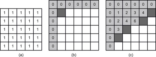 |
| Figure 33.10
A 2-D-wave approach to integral image calculation. Dark gray — N-th stage pixels, Light gray — already calculated values, White — yet not processed pixels. (a) Original image. (b) Initialization. (c) After a few iterations.
|
This algorithm, although simple to implement on the CPU, has some disadvantages when implementing it with CUDA:
1. It requires sparse nonlinear memory accesses.
2. It requires either several CUDA kernel launches (one for each slice of pixels) or a work pool, which in turn requires atomic operations on global memory.
A much better approach is to take into account the
separability
property of an integral image calculation (Table 33.7
), which means that it can be performed on all rows and then all columns of an image sequentially.
The algorithm that takes a vector
F
= [
a
0
,
a
1
, …,
a
n
− 1
] of length
n
and produces the vector
I
of length
n
+ 1 (refer to
Table 33.8
), where each element appears to be a sum of all elements of the input vector to the left, is known as
scan
or
prefix sums
.
It has a very efficient implementation for CUDA which can be found in the CUDPP library, Thrust library, and CUDA C SDK (“scan” code sample). Thus, the algorithm for integral image calculation is as follows:
1. Perform scan for all rows of the image
2. Transpose the result
3. Perform scan for all rows of the transposed scan (corresponding to columns of the original image)
4. Transpose the last result and write to the output integral image
It should be noted that unlike the input image, which has its pixel values typically stored in 8 bits, an integral image for the object detection task needs 32 bits per pixel to store the values. The exact amount of bits per pixel for storing an integral image can be easily calculated by evaluating the size of the largest rectangular region of original image pixels that will be ever summed. For example, if it is known a priori that the size of regions will always be less than 16 × 16, then a 16-bit data type can be chosen to store the integral image because the maximum sum (16 * 16 * 255 = 65280 = 0xFF00) doesn't overflow 16 bits. Hence, for searching large faces in 1080p video frames with a square object classifier, there is an obvious need of a 32-bit integer data type to store the integral image.
As for the squared integral image, which cannot fit into 32 bits, Intel decided to store its values in 64-bit floating-point type (see the
ippiRectStdDev
function). This creates an additional problem when we are implementing the algorithm on early NVIDIA CUDA architectures (SM < 1.3): G80, G84, G92, etc., which have no support for 64-bit double-precision floating-point values. The solution is to store squared integral image pixels in the 64-bit unsigned integer data type, which is supported by the CUDA-C compiler.
An efficient implementation of matrix transpose can be found in CUDA C SDK (“transpose” code sample).
Performing a scan for all rows/columns is a slightly different task compared with scanning of a single array. Launching scan
height
times to do scans of the image rows is not an efficient solution because a single row of an image doesn't contain enough data to provide sufficient workload for the device. This solution is also subject to additional time overhead caused by many API calls to the CUDA driver.
There are several ways to deal with a row-independent scan:
• CUDPP plans — an efficient tool for batching small similar tasks into the plan, which is then executed on the device. CUDPP takes care of optimal partitioning of the workload, if necessary.
• Thrust
exclusive_segmented_scan
function. This function, however, requires an additional array of the same type as the input image size. This array should be initialized with labels, indicating the beginning and end of each of the segments.
• Modify scan sample to work with independent rows in one kernel launch.
The modified scan kernel performs processing of an image row with one CUDA block; thus, the grid configuration contains
height
blocks (see example on
Figure 33.11
). Each CUDA block contains 128 threads, which perform (width
/
blockDim.x
) iterations along the image row. On every iteration threads load 128 elements from the row in global memory (gmem) into the shared memory (shmem), perform an exclusive scan, and add the carrier value to the prefix sums. The initial carrier value is set to zero,
but after the first iteration, it is updated with the sum of all elements being scanned up to the moment. Then the threads output values to the destination buffer in global memory.
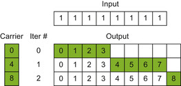 |
| Figure 33.11
A modified scan algorithm for integral image generation (four-thread CUDA blocks for the sake of clarity).
|
One of the best practices guidelines (included with CUDA toolkit documentation) states that a GPU must be provided with enough workload of the finest granularity. A good CUDA kernel doesn't change its behavior depending on the size of the input data; the input size has to be handled by means of CUDA block and grid configurations. It is claimed that in order to cover global memory access latency, each streaming multiprocessor (SM) should be able to keep about six CUDA blocks on the fly. Thus, to guarantee that the hardware is not wasting its resources while executing a kernel, the grid size of the kernel configuration must be greater than the maximum known number of SMs (30 on an NVIDIA GTX 280) multiplied by six, which gives the minimum sufficient image height of 180 pixels. As soon as the majority of multimedia content is stored in formats larger than CIF (352 × 288), the kernel demonstrates good performance on all known NVIDIA GPUs.
After we implement a set of kernels for integral image calculation, the next step is to implement the calculation of the squared integral image. Obviously, this new set of kernels is subject to code reuse, and it is likely possible to generate all integral image-related kernels by means of C++ templates. The differences between the scan kernels are listed as follows:
• The initial rowwise scan for the integral image: input data is unsigned 8 bit (u8
); output is unsigned 32 bit (u32
).
• The second rowwise scan for integral image: input is previously scanned and transposed data in
u32
; output is
u32
.
• The initial rowwise scan for the squared integral image: input data is
u8
, but the input pixels must be squared before passing into the scan. Output can be
u32
under the assumption that the row length (the input image maximum dimension) is sane and thus doesn't allow to overflow
u32
type.
• The second rowwise scan for the squared integral image: input data is
u32
; no squaring is needed. Output data is
u64
.
To implement this using C++ templates, three template parameters need to be introduced:
class T_in, class T_out,
and
bool bSquare
. The changing parts of the kernel are lines where the input image of type
T_in
is read into shared memory, where the value is squared after reading, and where the output is stored to the destination buffer of type
T_out
. To read the value from the source buffer of
u8
or
u32
type it is convenient to create the
__device__
function with the following signature:
template<class T>
static inline __device__ T readElem(T *d_src, Npp32u offs);
This function can have two explicit instantiations like below:
template<>
__device__ Npp8u readElem<Npp8u>(Npp8u *d_src, Npp32u offs)
{
return tex1Dfetch(texSrcNpp8u, offs);
}
template<>
__device__ Npp32u readElem<Npp32u>(Npp32u *d_src, Npp32u offs)
{
return d_src[offs];
}
33.3.2. Generation of the Normalization Values
As was mentioned previously, object classifiers are usually trained on the variance normalized data. To achieve this effect on the verification stage, one would need to calculate the pixels standard deviation of every region tested and divide each pixel value by the result.
The standard deviation of a rectangular region can be calculates from the formula in
Table 33.4
. For this, it requires four corner values of the region from the integral image and squared integral image, located either in global or texture memory.
The CUDA kernel configuration assumes a CUDA thread calculates one pixel of the normalization map, corresponding to the top-left corner of the
M
×
N
region of the original image. The configuration of CUDA block is not important unless it is possible to prefetch integral and squared integral images values by means of shared memory. For this purpose the block configuration is chosen as linear, 128 × 1 threads, and the shared memory of (128 +
N
− 1) × 2 elements of type
u64
are allocated. Before launch,
N
should be checked not to exceed the allowed amount of shared memory. This shmem segment is used for both integral images prefetching. The idea is to load elements from integral image and store in shmem in four copies: two for top and bottom 128 values and two for top and bottom
N
− 1 values. After that step, each thread addresses shared memory data four times at the correct corner positions and calculates the sum of pixels. The same applies to the squared integral image.
The calculation from
Table 33.4
deals with big numbers, representing sums of pixels and their squared values. Thus, all intermediate variables should have a data type sufficient to store intermediate values.
For the sum of pixel values,
u32
is sufficient for the square size less than 4096 × 4096 (to be precise, the maximum side is equal to sqrt(0xFFFFFFFF / 255)). The maximum squared pixels region has the side equal to sqrt(0xFFFFFFFF / 255^2) = 257, which is not enough for HD media content, and hence,
u64
type is used.
Once the sum of pixels in the region (u32 sumPix
) and sum of the squared pixels in the region (u64 sqsumPix
) are calculated, the variance can be calculated using the formula from
Table 33.9
.
Here, both the terms require division by the number of pixels, or essentially the square of the rectangular region. If this were a constant depending only on the classifier window size (M
×
N
), then the simple solution would be to hard-code this division using multiplication and right shifts. But in practice the normalization values calculation has to be performed on every scale of the input image; thus,
numPix
stands for the classifier area, multiplied by the current scale parameter squared.
To avoid usage of division (either integer or float) in the CUDA kernel, the
invNumPix
value is passed as a parameter instead, which is the reciprocal of
numPix
, stored in the float 32-bit (f32
) data type. With this variable the right term calculation is performed in two multiplications, while the left term leaves few issues unsolved.
Neither the hardware nor the compiler supports multiplication of
u64
by
f32
. The compiler won't generate any warnings, but one should be aware of implicit type casts — the
u64
value will be cast to
f32
, and after that, the multiplication will happen. The result calculation may be corrupt if the high word of the input
u64
was not empty.
To overcome this problem there are two possible solutions:
• Use double precision on systems that provide support to it (starting GT200) just to calculate this product. For the
u64
you need casting to double (f64
), then the multiplication is done and the
f64
result can be stored in
u32
;
• Use two
f32
variables to operate on the
sqsumPix
variable. The first one is a result of conversion from
u64
to
f32
. The second is a correction value, which can be obtained by backward conversion of the
f32
result to
u64
and subtraction from the true value. The residual is then converted to
f32
. Thus, the original
u64
is represented by two
f32
words, and the multiplication can be performed using the distributive property of the operation. See the following code snippet:
Npp32f sqsum_val_base = __ull2float_rz(sqsum_val);
Npp64u sqsum_val_tmp1 = __float2ull_rz(sqsum_val_base);
Npp64u sqsum_val_tmp2 = sqsum_val - sqsum_val_tmp1;
Npp32f sqsum_val_residual = __ull2float_rn(sqsum_val_tmp2);
sqsum_val_base *= invNumPix;
sqsum_val_residual *= invNumPix;
Npp32f sqsum_val_res = sqsum_val_base + sqsum_val_residual;
This approach appears to be superior even compared with the native support of double-precision floating-point values on GT200 and Fermi architectures — the register consumption and the speed are much better.
One more technical pitfall is the usage of unions on SM 1.x architectures. Here, the unions are needed to provide texture-cached reading of the integral image (u32
) and squared integral image (u64
). As long as there is no valid texture reference to use with
u64
data type, the texture reference that is bound to the memory containing squared integral image is declared of
uint2
data type. When we are reading the element of squared integral image, there are several ways to get the
u64
value:
1.
union
{
Npp64u ui1x64;
uint2 ui2x32;
}
tmp;
tmp.ui2x32 = tex1Dfetch(texSqr64u, x);
return tmp.ui1x64;
2.
uint2 ui2x32 = tex1Dfetch(texSqr64u, x);
return *(Npp64u *)&ui2x32;
3.
uint2 ui2x32 = tex1Dfetch(texSqr64u, x);
return (((Npp64u)ui2x32.y) << 32) | ui2x32. x;
The first two ways lead the compiler to the excessive usage of local memory (lmem), because these approaches make use of casting of the structure types. Usage of local memory when not necessary has a pernicious effect on the kernel's performance, especially on the architectures without lmem cache. Thus the third approach appears to be optimal.
33.3.3. Working on the Range of Scales
OpenCV has two ways of handling an object search on different scales. The first way is scaling of the image: an image is downscaled by the current scaling factor; all integral images and the normalization maps are recomputed, and the object classifier is applied to the downscaled content as if it was working always on the identity scale. This is the most straightforward way and at the same time most precise and most computationally expensive.
The second OpenCV way is to scale the classifier. The input image as well as integral images remain intact all the way, but the
M
×
N
classifier window is upscaled by the current scaling factor. On every new scale the normalization map is updated according to the current window size, and the object detector is applied. The problem with this approach is that when upscaling the
M
×
N
classifier window by the real value, the features don't map to the pixels grid anymore. In order to prevent the precision loss that is due to coordinates rounding, the weights of all features in the classifier cascade have to be updated on every scale according to the changed area of the features’ rectangles.
Both ways have pros and cons. The first way doesn't require changing the object classifier after its loading; it doesn't have problems with drifted feature area values, which may lead to the worse detection rate. However, it requires reconstructing the whole frame helper structures on every scale, which is a rather expensive operation. The second way needs to recalculate only the normalization map and adjust the classifier weights.
For the GPU implementation of the pipeline, one of the most important decisions to make is the data layout organization. The global memory access latency can be covered in several ways: access coalescing for direct access and spatial locality of adjacent accesses for cached access; it can be either texture cache or L1/L2 cache starting with Fermi architecture. The second approach doesn't fit into these requirements because with the growing scale factor, the distance between the adjacent accesses will only grow. The result is that such accesses can never be coalesced, and they also cause cache trashing. A limited amount of cache lines appear to be irrationally consumed to store one or a few elements of interest per line as shown in
Figure 33.12
.
 |
| Figure 33.12
Cache trashing when addressing sparse pixels (cache line size is 4 pixels width for clarity). White points represent sparse accesses, black points stand for unused cached pixels in cache lines.
|
The cons of the first way can be fought by the decision to work with only integer scales of the original image. This is the most valuable difference between the OpenCV processing pipeline and the one implemented with CUDA. The most tangible negative effect of this simplification is observed on the lowest scales, close to the identity. This implies worse detection rates for smallest faces. This should not be a big deal for the majority of applications that require only the largest face to be found.
Table 33.10
contains two series of scaling factors from the OpenCV algorithm and from the algorithm for CUDA. As can be seen, the scaling factors do not differ too much after a few scale iterations.
Downscaling with an integer factor is essentially a decimation of the input, or nearest neighbor downsampling — a process, in which the output buffer receives one sample per
N
original samples.
The next step is implementation of the CUDA kernel that performs the processing of a region of pixels at the original scale using the whole classifiers cascade. The kernel receives the classifier cascade, integral and squared integral images, normalization map, and a pointer to a segment of global memory where the output of classification is stored.
The very simplistic implementation of such a kernel has a simple mapping of the processing flow to CUDA grid and block configurations. The kernel is launched with as many threads as there are regions of the
M
×
N
size to be classified in the image, that is (height
−
M
+ 1) × (width
−
N
+ 1). Each CUDA thread works within the search region and sequentially calculates stages, classifiers, and features until the classification decision is done. After that it outputs the decision flag to the output detections mask of the same size as the input image.
The output mask should have a low amount of detections, so for the convenience of iteration over them, they are collected into the list of detections using the stream compaction algorithm.
Stream compaction is a data manipulation primitive that can be found in both CUDPP and Thrust libraries (in the Stream Compaction and Reordering section). The algorithm takes the input vector of values and the compaction predicate, which indicates if an element from the input vector should be in the output or not. The algorithm then outputs the “compacted” vector of only those values for which the predicate evaluated to true.
There are plenty of variations of stream compaction, such as taking different arguments, working with predicates or stencil masks, and outputting input elements themselves or their offsets from the beginning of the input vector.
Figure 33.13
shows the process of stream compaction based on the scan operation.
 |
| Figure 33.13
Stream compaction for object detections. Top to bottom: Input vector of elements, white are of interest; the mask of elements of interest; the prefix sums vector of the mask of interest (contains output offsets of the elements of interest); the compacted vector.
|
The vector at the top contains integer elements; some of them are darkened which means that these elements are not of interest. The purpose of the algorithm is to take only elements of interest and put them into the new “compacted” vector in the following three steps:
• The mask of elements of interest is calculated. Each white element has 1 in the mask and all others have zeros.
• This mask is prefix summed, which produces a vector of addresses for where to put elements of interest.
• The compaction is then performed as a simple elementwise copy.
It has to be noted that under certain conditions if the input vector contains a very low amount of elements of interest, then the use of atomic operations on the global memory instead of scan may give better performance.
Processing Optimizations
The approach to the classifier cascade application with CUDA, which maps each region to one CUDA thread, is hereby called pixel-parallel processing (Figure 33.14
). The CUDA block configuration is chosen to be linear for convenience. As a convention, the anchor of an
M
×
N
region will be represented by the top-left pixel (the middle pixel on the illustrations 33.15). Because all regions have to be processed by the kernel, all threads within the CUDA block will address the region of the
M
× (blockDim.x
+
N
− 1) of the integral image. This leads to the idea that any kind of cache would be extremely helpful here for prefetching of the integral image values. The possibilities are shared memory, texture cache, and L1/L2 cache (starting with the Fermi architecture). As for shared memory, it will not be efficient on early architectures owing to the ratio of shared memory per multiprocessor to the amount of threads to launch.
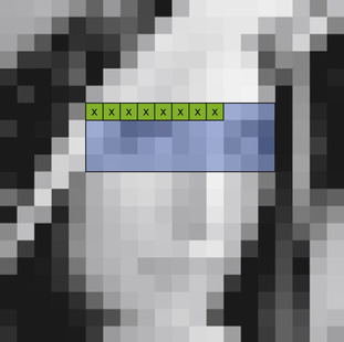 |
| Figure 33.14
Pixel-parallel processing (x-marked pixels are anchors, corresponding to CUDA threads; the rectangular area of pixels is shared by all threads of the block). The CUDA block size is eight threads, M = N = 4.
|
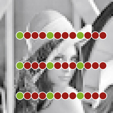
The described processing is very simple to implement, but its performance is below any expectations. The reason for this phenomenon is so-called work starvation. Indeed, on each stage the classifier cascade is supposed to reject some percentage of the input hypotheses, which means that just after a few stages more than 50% of CUDA threads will become inactive (Figure 33.15
). After all threads from the block terminate, the SM releases the CUDA block and its resources and proceeds with the new one. The worst-case scenario can happen if every CUDA block has one or more threads that will be discarded on the last stage of the cascade.
 |
| Figure 33.15
Lena image (bottom right) and masks of regions that passed through the first, second, third, sixth, and 20th stages of the face detection cascade.
|
The efficiency of the processing may be improved if the classifier cascade is broken down into groups of stages (or even into separate classifiers), which are then executed in sequential kernel launches. The kernel needs to be modified to take the amount of stages to process before forced termination. This idea draws several problems that have to be overcome.
Configuring CUDA blocks for subsequent launches as before doesn't make work starvation go away because the same threads are addressing the same regions. This problem can be dealt with by means of the stream compaction algorithm that is applied to the output mask of detections after the first group of stages processing; it is capable of creating a list with indices of those anchors which passed through.
As a result, there is a need in some other kernel for the subsequent launches that takes the list of indices as an argument and assigns one thread per anchor passed to the moment. This new kernel differs from the previous in several ways. Instead of the direct computing of the anchor location from
threadIdx
and
blockIdx
, the new kernel has a one-dimensional block configuration and takes the anchor from the list (passed as input) at the absolute thread
ID
in the grid. In addition, the kernel can output detections to the same locations of the output vector, relying on the compaction kernel, or it can do compaction by itself (either each thread increments a global counter using
atomicAdd
and writes
to the slot, or the local compaction stage is held after all threads finish classification and the atomic operation is called only once from the CUDA block to reserve the needed amount of detections in the global array).
Although the latter processing scheme allows one to keep work starvation under the control, the situation can still be improved by revisiting the parallelism of the CUDA implementation. The two disadvantages of the latter CUDA kernel are
• The adjacent threads within the CUDA block share little (or don't share at all) areas of corresponding regions; hence, the access pattern to the integral image is quite sparse; and
• The work starvation at a smaller scale remains in place: still a possibility exists that all threads but one will reject the anchor and exit immediately, while the one left will do processing up to the end.
The proposed new scheme is called stage-parallel processing (Figure 33.16
), which means that the parallelism has moved inside of the single-stage processing. The whole linear CUDA block is working
with one region, and the processing of one classifier stage is performed in the following way. If we assume that the stage contains more weak classifiers than the value of CUDA block dimension, each CUDA thread picks one corresponding weak classifier from the beginning of the stage and calculates its value for the given region. Then it accumulates the value in the register and advances to the next weak classifier, located
blockDim.x
weak classifiers apart. When all weak classifiers are evaluated, all threads perform parallel reduction of the local accumulators, which results in the stage value, which in turn is compared with the stage threshold, and the classification decision is made.
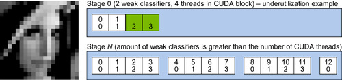 |
| Figure 33.16
Stage-parallel processing. One region 20 × 20 is processed by the whole CUDA block. Each white square represents one weak classifier with the absolute number in stage in the top field. The corresponding CUDA thread ID is in the bottom field.
|
The main advantage of this new kernel is the finest-grain parallelism, which completely solves the problem of work starvation and sparse memory accesses. It is also a disadvantage at the same time because the kernel is efficient only on the second part of the classifier cascade, where stages contain a large number of weak classifiers. Obviously, the performance of the kernel is low on the first stage of the face detection classifier cascade with a few weak classifiers.
The pros and cons of the two presented approaches certainly dictate the majority of usage restrictions. First, the pixel-parallel kernel executes several stages in one or a few launches. After that the stage-parallel kernel executes all hypotheses left up to the final classification. A good discussion topic would be “how to break down the cascade into groups of stages.” As before, here is the bifurcation point:
• The analytical way is to hard-code the decision based on the information about each classifier cascade. For instance, switch to the stage-parallel kernel after the ratio of passed anchors goes below some percentage threshold. This kind of information can be obtained on the cascade-training phase or calculated from an exhaustive amount of tests.
• The formal way is to switch to the stage-parallel kernel as soon as the amount of weak classifiers becomes greater or equal to the number of threads with which the stage-parallel kernel is configured to run.
• The feedback way is to call the pixel-parallel kernel restricted to process
N
(parameter to tweak) stages at a time several times until the percentage of passed hypotheses goes below the threshold, or the amount of weak classifiers on the next stage is greater than the stage-parallel kernel block dimension. In this case the first pixel-parallel kernel works in the very traditional way and outputs the hypotheses count and the list of detections (or the mask, and then the host calls the compaction operation to generate the list). All subsequent pixel-parallel calls take input from the list, generated
by the previous kernel call (so-called kernel chaining). The feedback analysis is performed on the host by copying the hypotheses count value and comparing it against the total number of possible detections. Whenever it becomes possible to do the feedback analysis on the device and call the next kernel depending on some condition directly from the device, then it should work a bit faster.
In every particular case (the classifier cascade) the fastest way needs to be determined, but in general the feedback way is superior owing to its robust essence.
Cascade Layout Optimizations
The object classifier cascade is the cornerstone of the object-detection pipeline. It is the most intensively addressed structure, and thus it has to be stored in a compact but well-structured representation. The OpenCV XML classifier representation (Table 33.11
) doesn't meet these requirements; its main purpose is to store the cascade in a pictorial, convenient for browsing way. In the OpenCV Haar classifier loader it is parsed to bits and stored in the RAM. The cascade structures being used in OpenCV after XML parsing can be found in the
cv.hpp
file. Although the internal representation is a structure of arrays that is an encouraged technique in GPU computing, there is still a lot of room for optimizations, especially GPU-specific.
The classifier adds up from stages, which in turn add up from trees (weak classifiers). Each tree consists of nodes, which encapsulate a number of rectangles with weights (the Haar feature), the feature threshold, and leaves. In
Table 33.11
the leaves are the weak classifier response values. To store the tree-based classifier, the
left_val
and
right_val
tags might be changed to
left_node
and
right_node
, with the
ID
of the referenced node instead of the classifier response.
To facilitate caching of the whole classifier cascade data, it needs to be stored in the global memory with texture reference bound to it. It is worth noting that texture reference supports reading up to 16-byte (128-bit) data types (e.g.,
uint4
), so the best approach is to pack the data to fit several arrays of structures (with elements of either 32, 64, or 128 bits in size), or to store it as several arrays of independent values.
Fortunately, all structures can be packed into the mentioned data types, not without hacks, though. The first array contains all feature rectangles with weights (Figure 33.17
). As far as an average classifier window size does not exceed some value in any dimension, the rectangle's fields (top, left, width, height) can be stored in 8-bit unsigned integers. The weight is stored as a single-precision floating point, so the overall size of the rectangle with weight is 64 bits. The corresponding structure is named
HaarFeaturePart64
.
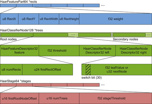 |
| Figure 33.17
Classifier cascade GPU data layout.
|
The second array contains descriptions of nodes. Each node is represented by the complete Haar feature, threshold, and two leaves (or pointers to other nodes). Because there are two leaves and one threshold, each stored as a 32-bit float (the leaf field can be interpreted as a 32-bit pointer to an other node, which agrees with the leaf size), this immediately leaves the only chance to fit “the complete Haar feature” into 32 bits to not exceed the allowed 128 bits for the total structure size. For this purpose the
HaarFeatureDescriptor32
structure is introduced. It contains the information about the number of rectangles in the feature (8 bits) and the offset from the beginning of the array of
HaarFeaturePart64
(24 bits). The whole 128-bit structure gets named
HaarClassifierNode128
.
It is important to store
HaarFeaturePart64
elements exactly in the same order as they appeared during the XML cascade parsing, because the
HaarFeatureDescriptor32
relies on their sequential order.
The final (third) array contains the description of the stages. Generally, a stage is characterized by the trees it contains and the stage threshold. The proposed representation of the stage is 16 bits for the amount of trees, 16 bits for the offset of the first tree root node in the array of
Haar-ClassifierNode128
, and 32 bits for the stage threshold. The corresponding data structure is named
HaarStage64
.
The
HaarStage64
representation relies on the solid indexing of the trees in the array of
Haar-ClassifierNode128
. Unlike the requirement of sequential filling of the array of
Haar-FeaturePart64
, the array of
HaarClassifierNode128
has to be handled slightly differently. In its first part all root nodes of the whole cascade are stored. After the last root node all intermediate nodes and leaves follow.
This layout allows keeping the size of
HaarStage64
without maintaining additional information about trees indexing. The opposite side of this storage scheme is a slightly more complex loading process, which has to maintain two separate arrays of nodes: one for root nodes and one for all others. After all nodes are loaded into the separate arrays, all far pointers to other nodes need to be corrected by adding the length of the root nodes vector.
One more bit-twiddling hack is storing the information about how to interpret the children of the node, that is, whether the 32-bit value is a floating-point leaf or integer pointer to some other node. Storing the single bit in the lowest bit of the integer (which is the least significant bit of the floating-point value at the same time) changes detection rates resulting from the precision loss. The safe location for this additional bit would be the highest bit of exponent (bit number 31) because it is never used in the values of weak classifier response. The highest exponent bit is used only for values with modulus greater or equal than 2, which rarely happens in practice, unless the classifier was trained with normalized weights.
Another potential placement for the classifier cascade is CUDA's constant memory. It is known to be one of the fastest memory types available on the GPU. The classifier cascade can be easily moved from global memory to constant memory. However, this enhancement has some application limitations.
First of all, constant memory is efficient only when a single location is addressed by all threads within a warp; otherwise, warp serialization occurs. Obviously, the worst warp serialization will happen in the stage-parallel kernel because every thread addresses a different weak classifier; thus, the optimization is not applicable here. However, the pixel-parallel kernel meets the addressing requirements because all threads address the same parts of the cascade simultaneously. The warp serialization still may happen while processing with a tree-based classifier, when different threads follow different paths depending on the calculations. No problems with serialization should happen when working with stump-based classifiers because of a lack of branching below the root node.
However, it appeared to be impossible to store the traditional face detection classifier cascade into the constant memory because the representation described earlier in this chapter required about 80 KB, whereas the capacity of constant memory is 64 KB (the size of the XML classifier representation is over 1 MB).
It appears that there is still a room for compression of the classifier cascade to increase chances for them to fit into the constant memory. This specific optimization covers only classifiers of limited window size (M
×
N
). The core idea is that the array of HaarFeaturePart64 takes about half of the total
size of the classifier cascade and by crunching it into 32 bits it is possible to achieve ∼75% compression ratio. Two things need to be done: the first (trivial) is storing the rectangle weight in the IEEE 754 half float (16 bits).
The second step is to learn how to store a feature rectangle into 2 bytes. Because of the symmetry in the definition of rectangle [(x
,
width
), (y
,
height
)], the problem can be reduced to storing a tuple (x
,
width
) in one byte (B
), under the constraints from the
Table 33.12
.
| x ∈ [0, N − 1] |
| width ∈ [1, N ] |
| x + width ∈ [1, N ] |
The final step is to calculate the maximum
N
for which all possible tuples can be stored in 1 byte. The enumeration scheme for this is shown on
Figure 33.18
(left). The increasing sum of elements from 1 to
N
evaluates to (N
+ 1) *
N
/2, which yields the maximum for
N
equal to 22. This means that the maximum allowed classifier window size to use with this technique is 22 × 22 pixels.
 |
| Figure 33.18
Schemes of solid enumeration (coding) of tuples (x, width) for N = 4.
|
The enumeration scheme can be used for building the conversion between (x
,
width
) and
B
, but it would require a square root operation involved.
Figure 33.18
(right) demonstrates the alternative enumeration scheme for which a very simple conversion exists (see
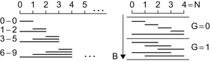
Table 33.13
). The idea is to restructure the enumeration into groups, each containing
N
+ 1 elements, and perform conversion with the use of intermediate values — the number of group in which the element is located (G
) and the number of element within the group (K
). On the tuple decoding step the division can be replaced with multiplication followed by arithmetic shifts, or multiplication by the precalculated reciprocal.
33.4. Benchmarking and Implementation Details
The CUDA implementation of the algorithm discussed in the preceding sections differs from OpenCV in several ways. For the sake of truthfulness of the comparison, the OpenCV 2.1 implementation of the function was prepared for the comparison as follows:
• Processing on the different scales was restricted to the rounded factors instead of the original approach.
• The initial region window size was set to the classifier window size.
• The “
ystep
” optimization was discarded because CUDA implementation processes all regions (this optimization forces the algorithm to skip processing every odd anchor along rows and columns if the current scale is less than 2, and results in 4 times less work on the particular scale).
• The library was compiled with Intel Threading Building Blocks support to enable the algorithm to use all CPU cores for parallel processing. OpenCV splits the image into horizontal slices and feeds them to the CPU cores, thus providing nearly 100% CPU load during processing.
• The amount of neighbors was set to 0 to exclude the hypotheses filtration stage from the processing time.
• Each image was loaded and processed several times to warm up command cache for the subsequent passes. The same was done for GPU processing.
All these restrictions are required to compare the algorithms, but in the real application, a lot of optimizations can be returned in place. For instance, when we are searching for the largest face, it is possible to early terminate after 10% of scales, providing a good speedup. All the optimizations reside on the top level of the pipeline, whereas the Haar classifier cascade application routine remains intact.
The results of the comparison can be found in
Figure 33.19
. The input data includes one group photo of large resolution, downsampled to several popular smaller resolutions (VGA, 720p, and 1080p). The hardware choice ranges from the low-end consumer GPUs and processors to the new high-end products. The plot demonstrates FPS (frames per second) of processing of each of the images by the selected GPUs and CPUs.
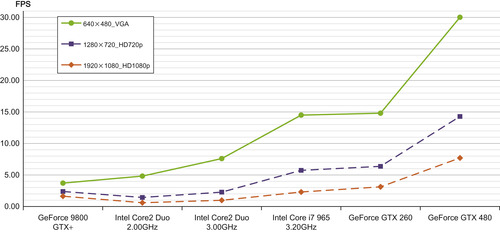 |
| Figure 33.19
Benchmarking of the GPU implementation against OpenCV library (Full search algorithm).
|
The ROC curve of the classifier should have not changed owing to the similarity of the results of OpenCV and GPU algorithms. All the discrepancies are studied and come from the difference between the hardware FP units and the order of floating-point operations.
Parts of the code are going to be available for free via OpenCV library GPU module. For questions regarding the chapter and the code send an email to the author.
At the time of active development of the classification-based object detection, Haar features appeared to be optimum of their computational complexity and the memory bandwidth, required for their computation. Since that time both compute capabilities and memory speed have grown, but the dynamics show that compute capabilities tend to grow faster.
Given this trend, the road map for creation of faster object detection algorithms for next-generation architectures should include revisiting of the low-level feature extraction algorithms and possibly changing simplistic Haar features to some higher-order correlation-based approach.
33.6. Conclusion
This gem has covered the history of the object detection approach, proposed by Viola and Jones. An efficient port of the object detection pipeline to NVIDIA CUDA architecture was presented, followed by a discussion of the implementation and possible sharp-tuned optimizations.
References
[1]
P.A. Viola, M.J. Jones,
Rapid object detection using a boosted cascade of simple features
,
In:
Proceedings of the 2001 IEEE Computer Society Conference on Computer Vision and Pattern Recognition (CVPR 2001)
,
vol. 1
(2001
)
Mitsubishi Electr. Res. Labs.
,
Cambridge, MA
, pp.
511
–
518
.
[2]
Y. Freund, R.E. Schapire,
A short introduction to boosting
,
In:
Proceedings of the Sixteenth International Joint Conference on Artificial Intelligence, AT&T Labs, Research Shannon Laboratory
Florham Park, NJ 07932 USA
. (1999
), pp.
771
–
780
.
[3]
R. Lienhart, J. Maydt,
An extended set of Haar-like features for rapid object detection
,
In:
IEEE ICIP 2002
,
vol. 1
(2002
)
Intel Labs., Intel Corp.
,
Santa Clara, CA
, pp.
900
–
903
.
[4]
R. Lienhart, A. Kuranov, V. Pisarevsky,
Empirical analysis of detection cascades of boosted classifiers for rapid object detection, MRL Technical Report
,
In:
DAGM'03, 25th Pattern Recognition Symposium
Madgeburg, Germany
. (2002
), pp.
297
–
304
;
(revised December 2002)
.
[5]
A. Obukhov,
Face detection with CUDA
,
In:
GPU Technology Conference
Fairmont Hotel, San Jose
. (2009
)
.
..................Content has been hidden....................
You can't read the all page of ebook, please click here login for view all page.