
Chapter 36. Image De-Mosaicing
Joe Stam and James Fung
36.1. Introduction, Problem Statement, and Context
Digital imaging systems include a lens and an image sensor. The lens forms an image on the image sensor plane. The image sensor contains an array of light-sensitive pixels, which produce a digital value indicative of the light photons accumulated on the pixel over the exposure time. Conventional image sensor arrays are sensitive to a broad range of light wavelengths, typically from about 350 to 1100 nm, and thus do not produce color images directly. Most color image sensors contain a patterned mosaic color filter array over the pixels such that each pixel is sensitive to light only in the red, blue, or green regions of the visible spectrum, and an IR cut filter is typically positioned in the optical path to reflect or absorb any light beyond about 780 nm, the limit of the human visible spectrum.
The typical mosaic or Bayer
[1]
pattern color filter array (CFA) is shown in
Figure 36.1
. This figure shows a common RG-GB configuration used throughout this example. Other arrangements may be used, including horizontal or vertical stripes rather than a mosaic. Different optical methods also exist to create color images, such as the common “three-chip” configuration used in some professional cameras where dichroic beam splitters direct three different spectral bands of the image onto three different image sensor arrays. Color-imaging techniques all have advantages with respect to image quality, cost, complexity, sensitivity, size, and weight. Although the merits of different color-imaging techniques may be hotly debated, the Bayer filter pattern has clearly emerged as the most popular technique for virtually all consumer and most professional video and still cameras.
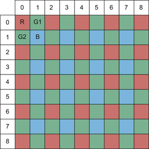 |
| Figure 36.1
Bayer pattern color filter array (CFA).
|
Because each pixel of a Bayer pattern filter responds to only one spectral band (red, green, or blue) the other two color components must be somehow computed from the neighboring pixels to create a full-color image. This process, commonly called
demosaicing,
or
de-Bayering
, is the subject of this chapter. Perhaps the simplest method is to reduce the effective resolution of the image by three quarters and treat each RG-GB 2 × 2 quad as a superpixel. Although simple, the lost resolution is undesirable, and artifacts remain because each pixel is not perfectly coincident with the other pixels in the quad. Many improved methods have been developed with various degrees of computational complexity. Simple linear interpolation between neighbors is probably the most commonly used, especially for video applications. Much more complex and higher-quality methods are preferred when postprocessing images from high-resolution digital still cameras on a PC — a tedious process typically referred to as RAW file conversion.
De-mosaicing occurs either by an embedded processor within a camera (or even on the image sensor chip) or as part of a postprocess step on a workstation after acquisition. Simple on-camera implementations result in a substantial loss of quality and information. Using a high-power processor would consume too much of the camera's battery life and produce heat and electrical noise that could degrade the image quality. Although on-camera methods are acceptable for consumer applications, professional photographers and videographers benefit from storing the raw unprocessed images and reserving the color interpolation for a later stage. This allows the use of much higher quality algorithms and prevents the loss of any original recorded information. Additionally, the user may freely adjust parameters or use different methods to achieve their preferred results. Unfortunately, the raw postprocessing step consumes significant computational resources, and thus, proves cumbersome and lacks fluid interactivity. To date, use of full high-performance raw conversion pipelines is largely limited to use for still photography. The same techniques could be used for video, but the huge pixel rates involved make such applications impractical.
Graphics processing units (GPUs) have become highly programmable and may be used for general-purpose massively parallel programming. De-mosaicing is such an
embarrassingly parallel
process ideally suited for implementation on the GPU. This chapter discusses implementation of a few de-mosaicing algorithms on GPUs using NVIDIA's CUDA GPU computing framework. The de-mosaicing methods presented are generally known and reasonably simple in order to present a basic parallel structure for implementing such algorithms on the GPU. Programmers interested in more sophisticated techniques may use these examples as starting points for their specific applications.
36.2. Core Method
Figure 36.2
shows a typical pipeline for the entire raw conversion process. First, each pixel from the image sensor produces a digital output, assumed to be a 16-bit integer number for this entire example. This raw measurement may need to be modified in a few different ways. First the black level (the digital value equivalent to having no signal on the pixel) must be subtracted. It is usually not 0, owing to biasing of the pixels at some voltage above the minimum range of the A/D converter and because there may be some spatially dependent offset, commonly called fixed-pattern noise. If the black level is spatially dependent, a row- and/or column-dependent lookup table provides the black level to subtract; otherwise, a constant value is used.
| Figure 36.2
The raw image conversion process pipeline.
|
After black-level compensation, the remaining signal is converted to a 32-bit floating-point value. For linear output sensors, simply scale to a 0.0-to-1.0 range by multiplying by the reciprocal of the white point value. If the output is nonlinear, then it must be converted through a function or a lookup table.
Next, the two missing color components are interpolated, the primary focus of this chapter discussed in detail. After interpolation the image must be adjusted for white balance and converted into the working color space. The color filter arrays on an image sensor are typically unique to a particular manufacturing process so the red, green, and blue values will not coincide with the color representation of a display or other standard color space. Simply multiplying the RGB components by a 3 × 3 matrix will suffice for this example, although more complex methods, such as a 3-D lookup table, provides more flexibility, particularly when dealing with out-of-gamut colors (for cameras capable of sensing colors outside the range of the chosen destination color space).
Numerous optional steps may be performed at this point such as denoising, sharpening, or other color adjustments. To stay concise, such enhancements are omitted from this sample, although the GPU is also very well suited for these tasks. Finally, the last stage applies a nonlinear gamma, if desired.
36.3. Algorithms, Implementations, and Evaluations
Obviously, a GPU implementation of de-mosaicing benefits from the massive parallelism of GPUs. Equally important to achieve high throughput is proper memory management and memory access patterns. Although GPUs have tremendous memory bandwidth, in excess of 100 Gb/s on the fastest cards, with the sheer amount of calculation necessary per pixel, the limit to achieve real-time performance is quickly surpassed when reading directly from uncached memory. Graphics shader programmers, on the other hand, will be familiar with using textures to read image data. Texture reads are cached and provide significant improvement over reading directly, but the cache size is limited, not under programmer control, and there is no provision for storing or sharing intermediate calculations without writing back to the GPU's external DRAM, or global memory (GMEM). In the CUDA architecture, NVIDIA added shared memory (SMEM), an extremely fast user-managed on-chip memory that can be shared by multiple threads. SMEM is perfect for storing source pixel information and will form the backbone of our de-mosaicing implementation.
The provided source contains implementations of GPU de-mosaicing using a few different methods: bilinear interpolation, Lanczos
[2]
interpolation, a gradient-modified interpolation
[3]
and the Patterned-Pixel Group method
[4]
. The particular details of the methods will be discussed later after a look at the overall application. Start by examining the file
main.cpp,
which contains a single
main()
function with the entire application control. The first step is to create an OpenGL window to display the output image. The details of OpenGL display or CUDA/OpenGL interop are beyond the scope of this chapter and are not discussed here
1
; a simple
CudaGLVideoWindow
class contains all the code necessary to draw the image on the screen.
1
CUDA/OpenGL interop is discussed in the NVIDIA CUDA Programming Guide. The user is also referred to a presentation entitled
What every CUDA programmer needs to know about OpenGL
from NVDIA'S 2009 GPU Technology Conference, available in the GTC 2009 archives at
.
Next, CPU memory is allocated to store the original raw image prior to transfer to the GPU. Pinned host memory, allocated with
cudaHostAlloc(),
is selected to facilitate fast, asynchronous DMA (Direct Memory Access) transfers of data to the GPU. In a real-time system, pinned memory would facilitate simultaneous data transfer and processing so that one frame could be processed, while the next frame is read and uploaded to the GPU. To avoid convoluting this sample with lots of file-parsing code, no attempt is made to read any standard raw file format; rather, several images are provided in a flat binary file, and all image properties are hard-coded above the declaration of
main().
Thus, users can easily replace this code with the necessary routines to acquire images from a particular source. Also, and consistent with our goal of simplicity, the sample implements only the common red-green1-green2-blue (or R-G1-G2-B) pixel arrangement shown in
Figure 36.1
. Best performance results when targeting the kernel to a specific pixel arrangement rather than including all the conditional logic to support possible variations.
The output image for this sample is an RGBA image with 32-bit/channel floating-point precision. GPUs efficiently handle 32-bit floating-point data, and this preserves the color precision and dynamic range of high-quality image sources; however, other output types are trivially substituted.
The quality of raw conversion algorithms is highly subjective. It is routinely debated, and depends on particular properties of specific cameras or the type of images acquired. Some algorithms, such as the PPG method, actually switch between calculations or vary coefficients based upon edge gradients or image content. Bilinear interpolation is chosen for simplicity and because it is regularly used when processing power is limited. Lanczos interpolation is also simple conceptually, but it provides superior output quality and can run on the GPU with only a modest decrease in throughput, despite a significant increase in overall computation load. The Malvar method
[3]
applies a gradient correction factor to the results of bilinear interpolation for dramatic improvement in quality with little additional complexity (and in this example we also apply the Malvar gradients to the Lanczos interpolation). Finally, the PPG method demonstrates a more complex conditional approach common in many of the most advanced de-mosaicing methods. This chapter does not advocate for the use of any particular method, or make claims about the comparative quality of different methods. Rather, this sample demonstrates the techniques to achieve high-performance de-mosaicing on an NVIDIA GPU, and developers can easily substitute their own preferred algorithms if desired (also see
[5]
).
The file
DeBayer.cu
contains the CUDA C kernels along with the kernel launch functions. Examine
DeBayer_Bilinear_16bit_RGGB_kernel(),
the bilinear de-mosaicing kernel. In this method, the missing color components for each pixel are computed from the average of the neighboring adjacent pixels of the other colors. More precisely refer to
Figure 36.3
and the following formulas:
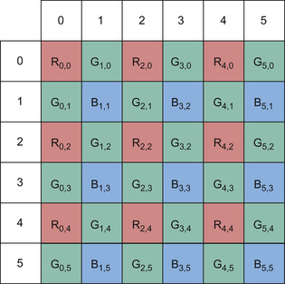 |
| Figure 36.3
Pixel computation layout.
|
For Red pixel
R
2,2
:

For Blue pixel
B
1,1
:

For Green Pixel
G
2,1
:
Each thread will process one 2 × 2 pixel quad and outputs four RGBA F32 pixels. This strategy prevents thread divergence that would occur if each thread processed one output pixel and applied different formulas. Two pixels are read once as a
ushort2
value by each thread. The first two steps of the pipeline of
Figure 36.2
are implemented in one simple code statement:
fval = CLAMP((float)((int)inPix.x − black_level) * scale, 0,1.0f);
In our example case the black level is assumed uniform across the image. As previously mentioned, the black level is commonly spatially dependent upon row or column location owing to fixed pattern noise from manufacturing variations in the row and column read-out circuitry and A/D converter variability in the image sensor. In this case the variable
black_level
may be replaced with a row or column lookup-table. The resulting integer value is then cast to float and multiplied by a predetermined
scale
variable to convert the value to floating point in the 0.0f to 1.0f range. Again, for simplicity, the source data is assumed linear; if it is not then a linearization function may be applied. In this case a 1-D CUDA texture provides an ideal way to implement a lookup table with hardware linear interpolation.
The linear scaled floating-point raw values are now stored in the GPU's shared memory (SMEM). SMEM is extremely fast on-chip memory accessible to all threads within a thread block. It is analogous to CPU cache memory, but allocated and accessed under programmer control and thus can be relied upon for deterministic performance. SMEM serves the needs of de-mosaicing perfectly because the multiple threads in a block need to access the same source raw pixel values.
The thread block size dictates the input tile size stored. Additional apron source pixels are needed to interpolate pixels at edges of the tile, so the source reads are shifted up one row and left two columns with the left two threads in the thread block reading extra columns and the top two thread rows reading extra rows (two extra columns are read on each side rather than the one needed to maintain 32-bit read alignment).
2
For the first generation of NVIDIA GPUs with compute capability 1.x, a thread block size of 32 × 13 requires 34 × 14 × 4 pixels, or 7616 bytes total, just less than 50% of the total 16 kilobytes of SMEM. Thus, two thread blocks run concurrently per SM, ensuring good overlap between memory access and computation. On the newest compute capability 2.x GPUs, 48 kB of SMEM is available, so a thread block size of 32 × 24 is chosen. SMEM is no longer the limiting factor; rather, 768 threads is 50% of the maximum 1572 threads per SM.
2
An observant programmer may notice that the global memory reads are not strictly aligned for proper coalescing; however, shifting the columns by one 32-bit word does not have a significant performance detriment, and further complication of the code is unwarranted. SM 1.2 and later architectures contain coalescing buffers or cache, thus eliminating the need for the complex read patterns needed to strictly coalesce memory.
Reading the source data and storing the values into SMEM compose the majority of the code in the sample, and unfortunately complicates the implementation quite a bit. The performance benefit far outweighs the complexity that arises from shifting the reads for the extra row and column apron pixels, and properly clamping on the image boarders. Also, note that the raw source pixels are stored in SMEM as four different color planes rather than a contiguous tile. This prevents a two-way SMEM bank conflict that would arise because every thread processes two output pixels per row. The arrangement of the source reading and storage in SMEM is shown in
Figure 36.4
. Also note that the blue and green-2 SMEM tiles contain one extra apron row on top and the red and green-1 tiles contain their extra apron row on bottom.
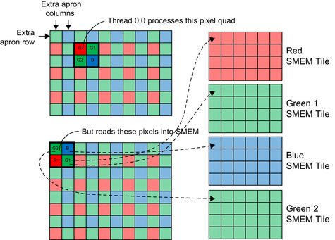 |
| Figure 36.4
Source reading and storage.
|
The overall read process is diagramed in
Figure 36.5
.
 |
| Figure 36.5
Read process.
|
The read process may also be understood by referring to the following pseudo code, which directly mirrors the code for the bilinear interpolation in the accompanying source code:
Pseudo Code for Bilinear Interpolation reads to SMEM
Notes:
X
is the two-pixel column index in the image (Reading two 16-bit pixels at a time).
References to ‘X’ or ‘Column’ below are two physical columns.
Y
is the row index.
Tx
and
Ty
are the thread indices.
Boundary checking for off-of-image reads are omitted in this pseudo code for clarity.
// Step 1: Read Green2 and Blue pixels for the top left part of the tile
// Reads are shifted up one row and left one double-column
Column = X − 1
Row = Y − 1
Pixels = Image[Row][Column]
Linearize and Scale Pixels
Green2_SMEM_Tile[Ty][Tx] = Pixels[0]
Blue_SMEM_Tile[Ty][Tx] = Pixel[1]
If Tx< 2
Columnextra Green2 and Blue pixels = X + Thread Block Width − 1
Pixels = Image[Row][Column]
Linearize and Scale Pixels
Green2_SMEM_Tile[Ty][Tx + Thread Block Width] = Pixels[0]
Blue_SMEM_Tile[Ty][Tx + Thread Block Width] = Pixel[1]
//Step 3: Read the Red and Green 1 pixels from the next row
Row = Y
Column = X − 1
Pixels = Image[Row][Column]
Linearize and Scale Pixels
Red_SMEM_Tile[Ty][Tx + Thread Block Width] = Pixels[0]
Green1_SMEM_Tile[Ty][Tx + Thread Block Width] = Pixel[1]
// Step 4: Read the extra Red and Green 1 pixels for the right apron
If Tx< 2
Column = X + Thread Block Width − 1
Pixels = Image[Row][Column]
Linearize and Scale Pixels
Green2_SMEM_Tile[Ty][Tx + Thread Block Width] = Pixels[0]
Blue_SMEM_Tile[Ty][Tx + Thread Block Width] = Pixel[1]
// Step 5: Need to read two rows on the bottom to complete the apron
If Ty < 2
Column = X − 1 Row = (BlockIdx.y + 1) + BlockHeight*2 + Ty − 1
Pixels = Image[Row][Column]
Linearize and Scale Pixels
If Ty = 0
Green2_SMEM_Tile[Ty + Thread Block Height][Tx] = Pixels[0]
Blue_SMEM_Tile[Ty + Thread Block Height][Tx] = Pixel[1]
If Ty = 1
Red_SMEM_Tile[Ty + Thread Block Height][Tx] = Pixels[0]
Green1_SMEM_Tile[Ty + Thread Block Height][Tx] = Pixel[1]
// Step 6: Read the bottom right apron pixels
If Ty < 2 and Tx< 2
Column = X + Thread Block Width − 1
Row = (BlockIdx.y + 1) + BlockHeight*2 + Ty − 1
Pixels = Image[Row][Column]
Linearize and Scale Pixels
If Ty = 0
Green2_SMEM_Tile[Ty + Thread Block Height][Tx + Thread Block Width] = Pixels[0]
Blue_SMEM_Tile[Ty + Thread Block Height][Tx + Thread Block Width] = Pixel[1]
If Ty = 1
Red_SMEM_Tile[Ty + Thread Block Height][Tx + Thread Block Width] = Pixels[0]
Green1_SMEM_Tile[Ty + Thread Block Height][Tx + Thread Block Width] = Pixel[1]
Following the reading from global memory into SMEM, each thread block must synchronize with a
__syncthreads()
call to ensure all reads are complete before continuing. For this reason, the block sizes discussed previously are chosen to allow two blocks to run per SM, thereby giving the GPU compute work to do on one block, while another reads and waits for synchronization.
After synchronization each thread computes the missing color components for each output pixel in the 2 × 2 quad according to the preceding formulas. The output RGB value for each pixel is multiplied by the 3 × color conversion matrix for the target output color space. More sophisticated color conversion methods, such as a 3-D lookup table using 3-D textures, may be substituted here to account for different rendering intent. Finally, the output gamma is applied and the result is clamped in the 0 to 1.0 range. Note that clamping may be omitted if out-of-gamut colors are permitted. Here is the CUDA-C code for the interpolation of additional color channels of the red filtered (northwest) pixel in the quad. The variables
tile_R, tile_G1, tile_G2
, and
tile_B
refer to the SMEM memory tiles containing the source pixel values for each color channel.
// Bilinear Interpolation
float4 NW;
NW.x = tile_R[sy][sx];
NW.y = 0.25f * (tile_G2[sy][sx] + tile_G2[sy+1][sx] +
tile_G1[sy][sx-1] + tile_G1[sy][sx]);
NW.z = 0.25f * (tile_B[sy][sx-1] + tile_B[sy][sx] +
tile_B[sy+1][sx-1] + tile_B[sy+1][sx]);
NW.w = 1.0f;
// color correction
float r = ColorMatrix[0] * NW.x + ColorMatrix[1] * NW.y + ColorMatrix[2] * NW.z;
float g = ColorMatrix[3] * NW.x + ColorMatrix[4] * NW.y + ColorMatrix[5] * NW.z;
float b = ColorMatrix[6] * NW.x + ColorMatrix[7] * NW.y + ColorMatrix[8] * NW.z;
// gamma
NW.x = CLAMP(__powf(r,gamma),0,1.0f);
NW.y = CLAMP(__powf(g,gamma),0,1.0f);
NW.z = CLAMP(__powf(b,gamma),0,1.0f);
// write output
pOut[Y*2*OutPitch_in_pixels + X*2] = NW;
Each thread writes each pixel of the 2 × 2 quad back out to GPU GMEM after computation is completed. Because each thread processes 2 pixels per row, only every other 128-bit word is written at a time, and strict coalescing does not occur. Alternatively, these values could be stored until the entire quad is processed, written back to SMEM (which can now be reused because the processing of the source raw data is complete), and then written to GMEM in a coalesced fashion. Experimentally, it has been determined that just writing the values immediately performs better because the writes of the first 3 pixels per thread can overlap the processing of the subsequent pixels. It is quite common to perform sharpening, noise reduction, or other color adjustments as part of the raw conversion process. After interpolation pixels may be stored back to the now free SMEM and filters applied. Performing this processing may be more efficient than running a separate kernel later because extra passes through GMEM are eliminated.
3
When all additional filtering completes, then apply the final color conversion and gamma.
3
The benefit of concatenating additional filtering into the de-mosaicing kernel is heavily dependent on the complexity of the additional operations. For computationally intensive filtering, the memory latency may be hidden by computation, and thus, breaking filters into separate kernels may prove easier to code and manage. For simple filters or additional color adjustments, memory latency and bandwidth constraints will bottleneck performance, and thus, adding the filter to the de-mosaicing kernel will likely provide superior performance.
36.3.1. Improved Filtering
Bilinear interpolation leaves much to be desired in image quality that is especially noticeable at the edges in images. It is quickly evident that only a small portion of the kernel code in the preceding example relates to the actual interpolation computation, so presumably more complex methods may be used without a substantial performance penalty. Here, we discuss additional methods that improve upon the quality of the bilinear interpolation kernel.
In the sample, a second kernel,
DeBayer_Lanczos_16bit_RGGB_kernel()
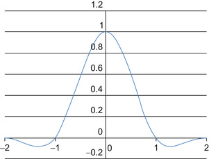
, implements Lanczos interpolation. Lanczos interpolation is regarded as one of the highest-quality methods of image resampling. Coefficients for the Lanczos operator are given by:
 Where
x
is the distance between each pixel in the neighborhood and the interpolated location and
a
is the order of the filter (a = 2 in our example). A plot of the Lanczos function is shown in
Figure 36.6
.
Where
x
is the distance between each pixel in the neighborhood and the interpolated location and
a
is the order of the filter (a = 2 in our example). A plot of the Lanczos function is shown in
Figure 36.6
.
 |
| Figure 36.6
Plot of the Lanczos 2 function.
|
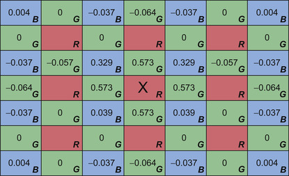
To interpolate the missing color values for each pixel compute a weighted sum of the neighboring pixels filtered in the desired color. The weights are the product of the x and y Lanczos function values for the distance between the output pixel and the neighbors in each axis. Consider interpolating the blue and green color values for a red filtered pixel.
Figure 36.7
shows the weights by which the neighboring green and blue pixels are multiplied and then summed to compute the corresponding blue and green color values. The sum is then normalized by multiplying by the reciprocal of the sum of the weights.
 |
| Figure 36.7
Lanzcos filter coefficients.
|
The Lanzcos interpolation CUDA kernel function is similar to the bilinear interpolation kernel, with the following substantial differences:
• A wider apron read is necessary to accommodate the larger neighborhood used to compute the interpolated values; thus, three extra rows above and below and four extra columns right and left are read. Because of the larger apron more SMEM is required, and thus, a smaller block size is used.
• The actual interpolation computation involves using several more input pixels and coefficients for each output pixel, but otherwise, follows the form for the bilinar kernel.
The CUDA-C code for computing the interpolated values of a red filtered pixel is as follows:
// Lanczos Interpolation
NW.x = tile_R[sy][sx];
NW.y = (−0.063684f * tile_G2[sy-1][sx] +
0.573159f * tile_G2[sy][sx] +
-0.063684f * tile_G1[sy][sx-2] + 0.573159f * tile_G1[sy][sx-1] +
0.573159f * tile_G1[sy][sx] + −0.063684f * tile_G1[sy][sx+1] +
0.573159f * tile_G2[sy+1][sx] + −0.063684f * tile_G2[sy+2][sx])
* 0.490701f;
NW.z = (0.004056f * tile_B[sy-1][sx-2] + −0.036501f * tile_B[sy-1][sx-1] +
-0.036501f * tile_B[sy-1][sx] + 0.004056f * tile_B[sy-1][sx+1] +
-0.036501f * tile_B[sy][sx-2] + 0.328511f * tile_B[sy][sx-1] +
0.328511f * tile_B[sy][sx] + −0.036501f * tile_B[sy][sx+1] +
0.328511f * tile_B[sy+1][sx] + −0.036501f * tile_B[sy+1][sx+1] +
0.004056f * tile_B[sy-2][sx-2] + −0.047964f * tile_B[sy+2][sx-1] +
-0.047964f * tile_B[sy+2][sx] + 0.004056f * tile_B[sy+2][sx+1]) * 0.963151f;
NW.w = 1.0f;
Malvar, He, and Cutler improved upon basic interopolation by including a gradient-correction gain factor that exploits the correlation between the red, green, and blue channels in an image. A weighted luminance gradient of the actual filter color for each pixel is added to the output of the interpolated missing color. The specific gradient correction gain calculation forumulas for each particular interpolation case are given in
[3]
and in the accompanying source code. The gain correction factor uses an additional 5 to 9 additional pixel values in the calcualtion of the final interpolated color. However, because these values are already located in SMEM, the overall performance of the calcualtion is remarkably close to simple bilinear interpolation. We now list the calculation of the output of a red filtered pixel for comparison with the previously listed methods.
// Bilinear Interpolation + Gradient Gain Correction Factor
NW.x = tile_R[sy][sx];
NW.y = 0.25f * (tile_G2[sy][sx] + tile_G2[sy+1][sx]
+ tile_G1[sy][sx-1] + tile_G1[sy][sx]) + 0.5f * tile_R[sy][sx] +
-0.125f * (tile_R[sy-1][sx] + tile_R[sy+1][sx] + tile_R[sy][sx-1]
+ tile_R[sy][sx+1]);
NW.z = 0.25f * (tile_B[sy][sx-1] + tile_B[sy][sx] + tile_B[sy+1][sx-1]
+ tile_B[sy+1][sx]) + 0.75f * tile_R[sy][sx] +
-0.1875f * (tile_R[sy-1][sx] + tile_R[sy+1][sx] + tile_R[sy][sx-1]
+ tile_R[sy][sx+1]);
NW.w = 1.0f;
The Patterned Pixel gGrouping (PPgG) algorithm is used to interpolate red (R), green (G), and blue (B) values at each location, just as in the previous discussions, although the algorithm differs from the previous examples. PPG performs a two-phase computation that begins by interpolating all missing green values. For interpolation of the green values at blue or red pixels consider estimating
G
2,2
at
R
2
2
. First, the method calculates gradients in four directions, centered at pixel
R
2
2
:
Next, the algorithm determines which direction has the minimum gradient and then uses that direction to estimate green values at the red locations, such as at
G
2,2
, as:
This fully fills in the green channel at all locations, and those results can now be used in the next steps. For interpolation of the blue and red values at green pixels, the algorithm estimates
B
2,1
and
R
2,1
at
G
2,1
by a “hue transit” function, given a set of inputs:
 where hue_;transit() is defined as:
hue_transit(l
1
,
l
2
,
l
3
,
v
1
,
v
3
){
if (l
1
<
l
2
<
l
3
||
l
1
>
l
2
>
l
3
)
return(v
1
+ (v
3
−
v
1
) × (l
2
×
l
1
)/(l
3
×
l
1
)
else
return(v
1
+
v
3
)/2 + (l
2
× 2 −
l
1
−
l
3
)/4
}
Finally, for interpolation of the blue or red values at red or blue pixels, consider estimating
B
2,2
at
R
2,2
:

Then, the final values for
B
2,2
and
R
2,2
are determined as:
if Δne ≤ Δnw
B
2,2
= hue_transit(G
3,2
,
G
2,2
,
G
1,3
,
G
3,2
,
G
1,3
)
else
B
2,2
= hue_transit(G
1,1
,
G
2,2
,
G
3,3
,
G
1,1
,
G
3,3
)
Each pixel processed in the PPG method is dependent only on a neighborhood of pixels around it. As in the previous examples, multiple reads and writes are issued to this neighborhood, and it can be stored in shared memory for faster repeated read access. In the case of PPG, the size of the region must be somewhat extended to accommodate for generating apron green values to avoid any need for a global synchronization (which would require a new kernel launch).
A tile of Bayer data and surrounding apron region can be copied from global memory into shared memory, and a group of threads can process a tile. If the CUDA-C algorithm was written to have each thread process a single element of the Bayer pattern, this would result in divergence because the operations to interpolate values for different colors vary at each location. So, as in the previous methods, the algorithm can be written so that each thread is responsible for processing a 2 × 2 region of the data corresponding to a “quad” of four data element locations: {
R
1
G
1
B
1
G
} = {
R
0,0
,
G
1,0
,
B
1,1
,
G
0,1
}. This way, all threads execute interpolations for
R
0,0
, then
G
1,0
, and so on, and so avoid divergent paths.
The PPG algorithms require substantially more SMEM than the prior methods for storing the interpolated green values from phase 1, and bank conflicts must again be avoided. Thus, for PPG analysis, we examined an alternative case where the input data is stored in SMEM as 16-bit short integer data. Linearization and black-level subtraction may still be performed upon the read of the raw data, but then values are converted back to short integers to conserve SMEM. Conveniently, when 16-bit source Bayer pattern values are written into shared memory and with each thread processing a “quad” of data, it can be seen that successive threads will each access different and successive banks of shared memory. This is a result of the banks accommodating two 16-bit elements per bank, and a row of Bayer data consisting of two 16-bit elements per “quad” element on a row, meaning the next quad's
R
1
value is spaced 32 bits, or one bank, away from the previous quad's
R
1
value, and so on. Thus, operating on 2 × 2 regions of 16-bit elements avoids divergence and bank conflicts. Finally, as seen in the preceding formulas the PPG method does not require any computation with precise floating-point weights; all calculations use integer math. Thus, the entire calculation and final output are written using unsigned short values.
36.4. Final Evaluation
Image de-mosaicing is extremely well suited for implementation on a graphics processor using NVIDIA CUDA. Several example algorithms are provided and serve as a framework that can be easily modified to suit a specific requirement.
Table 36.1
summarizes performance for several of the methods tested on an NVIDIA Quadro 5000 GPU. These metrics include timing of the entire raw conversion process outlined in
Figure 36.2
, which includes the final output color correction and write to memory as a full 32-bit float per color channel image. Timing does not include data transfer or drawing time because such requirements vary significantly for each application, transfer can likely be overlapped with computation, or live video feeds may be captured direct to GPU memory.
| Method | Pixel Rate |
|---|---|
| Bilinear | 2.1 Gpixels/s |
| Lanczos | 1.7 Gpixels/s |
| Malvar | 1.9 Gpixels/s |
| Lanczos + Malvar | 1.6 Gpixels/s |
Such performance is easily sufficient for real-time high-quality demosaicing results on high-resolution images. In fact, at such rates even a stereo pair of ultra-high-definition 4K video images can be processed in real time on a single GPU. Use of the GPU's shared memory facilitates such high performance by making neighboring pixel values instantly available for computation. Because of the shared memory and the GPU's overall high-computation performance, complex and high-quality methods require only slightly more computation time than simple methods. For example, the Lanczos method runs only about 25% slower than simple bilinear interpolation, despite an approximately fourfold increase in calculation. Finally,
Figure 36.8
shows the quality of each of these algoirthms in some particularly troublesome regions of test images from the Kodak test suite
[6]
.
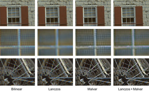 |
| Figure 36.8
Results comparison on standard.
|
References
[1]
B.E. Bayer, U.S. Patent 3,971,065, 1975.
[2]
C.E. Tarjan,
Lanczos filtering in one and two dimensions
,
J. Appl. Meteor.
18
(1979
)
1016
–
1022
.
[3]
H.S. Malvar, L.-W. He, R. Cutler,
High-quality linear interpolation for demosaicing of Bayer-patterned color images, Microsoft Research
(2004
)
.
[4]
C.K. Lin,
Pixel grouping for color filter array demosaicing
,
http://web.cecs.pdx.edu/~cklin/demosaic/
.
[5]
A. Lukin, D. Tarjan,
High-quality algorithm for Bayer pattern interpolation
,
Program. Comput. Software
30
(6
) (2004
)
347
–
358
.
[6]
B.K. Gunturk, Y. Altunbasak, R.M. Merseau,
Color plane interpolation using alternating projections
,
IEEE Trans. Image Process
11
(2002
)
997
–
1013
.
[7]
M. Tarjan,
Efficent, high-quality Bayer demosaic filtering on GPUs
,
submitted to J. Graph. GPU Game Tools
13
(4
) (2009
)
1
–
16
.
..................Content has been hidden....................
You can't read the all page of ebook, please click here login for view all page.